


Man AHL has recently published a research piece titled “A Trend Following Deep Dive: Cash (Equities) Is King” (Panjabi, Bordigoni, and Buchanan, 2026) which has resonated not only with researchers in the trend-following space but also with those specializing in equity markets.
The authors show that cross-sectional momentum techniques can be successfully applied across equity-style factors, potentially providing meaningful diversification relative to traditional time-series approaches.
In practical terms, an investor who already holds a conventional trend-following allocation across asset classes may benefit from adding a more orthogonal source of return: going long the strongest-performing equity factors while shorting the weakest-performing ones.
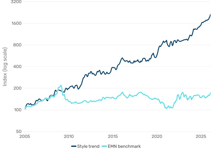
The chart below illustrates the equity curve of the style-trend portfolio presented by Man AHL.
Needless to say, our team found the piece sufficiently insightful to warrant further investigation.
In this article, we extend the analysis using Professor Kenneth French’s publicly available data library for U.S. equity factors.
We divide the sample into two adjacent periods: 1985–2005 and 2006–2026. The latter closely matches the period studied by Man AHL, while the preceding 20 years provide a useful historical comparison. The earlier sample can also be interpreted as broadly in-sample-like, since many of the underlying anomalies were discovered or popularized using data from that period.
As is often the case with studies based on academic factor portfolios, the results should not be interpreted as a ready-to-trade investment strategy. In our view, however, they highlight (and confirm) several findings that may be valuable when constructing actively managed, factor-based equity portfolios.

Factor Portfolio Construction
For our analysis, all data are sourced from Professor Kenneth French’s Data Library, one of the most widely used standards in academic factor research. The portal hosts hundreds of datasets covering portfolios formed on firm characteristics, industry groupings, and other classifications.
Readers who are new may find the Concretum Factor Tracker useful. It is a free tool we built to conveniently collect, track and visualize several US equity factor portfolios from the French library.

Factors are typically constructed as long-short exposures to decile portfolios. For each characteristic (such as value, momentum, or profitability) stocks are sorted into ten portfolios, or “deciles,” according to their ranking on the selected signal.
One important design choice concerns the weighting scheme within each decile portfolio. Stocks can be equally weighted, assigning the same weight to every constituent, or value weighted, with larger companies receiving proportionally greater weights based on market capitalization. Since both approaches are widely used in academia and practice, we examine them separately throughout the study.
As a convention, we identify D10 as the decile that historically earns the documented premium and D1 as the opposite extreme, flipping the source labels where necessary: each factor is therefore constructed as a long position in D10 and a short position in D1.
A second design choice concerns how the two legs are combined into a long-short factor portfolio.
One common approach is dollar-neutral weighting, where each decile carries 100% notional exposure, giving the combined portfolio 200% gross exposure.
Another widely used approach is volatility scaling, under which each leg is resized periodically to target a predefined level of volatility. Because the realized volatility of D10 and D1 can differ substantially, scaling the two legs independently prevents the more volatile side from dominating the portfolio’s total risk.
Unless otherwise stated, this study adopts the second approach and assigns the same volatility target to both legs (see “Momentum Has Its Moments” by Barroso and Santa-Clara (2015) for additional discussion).
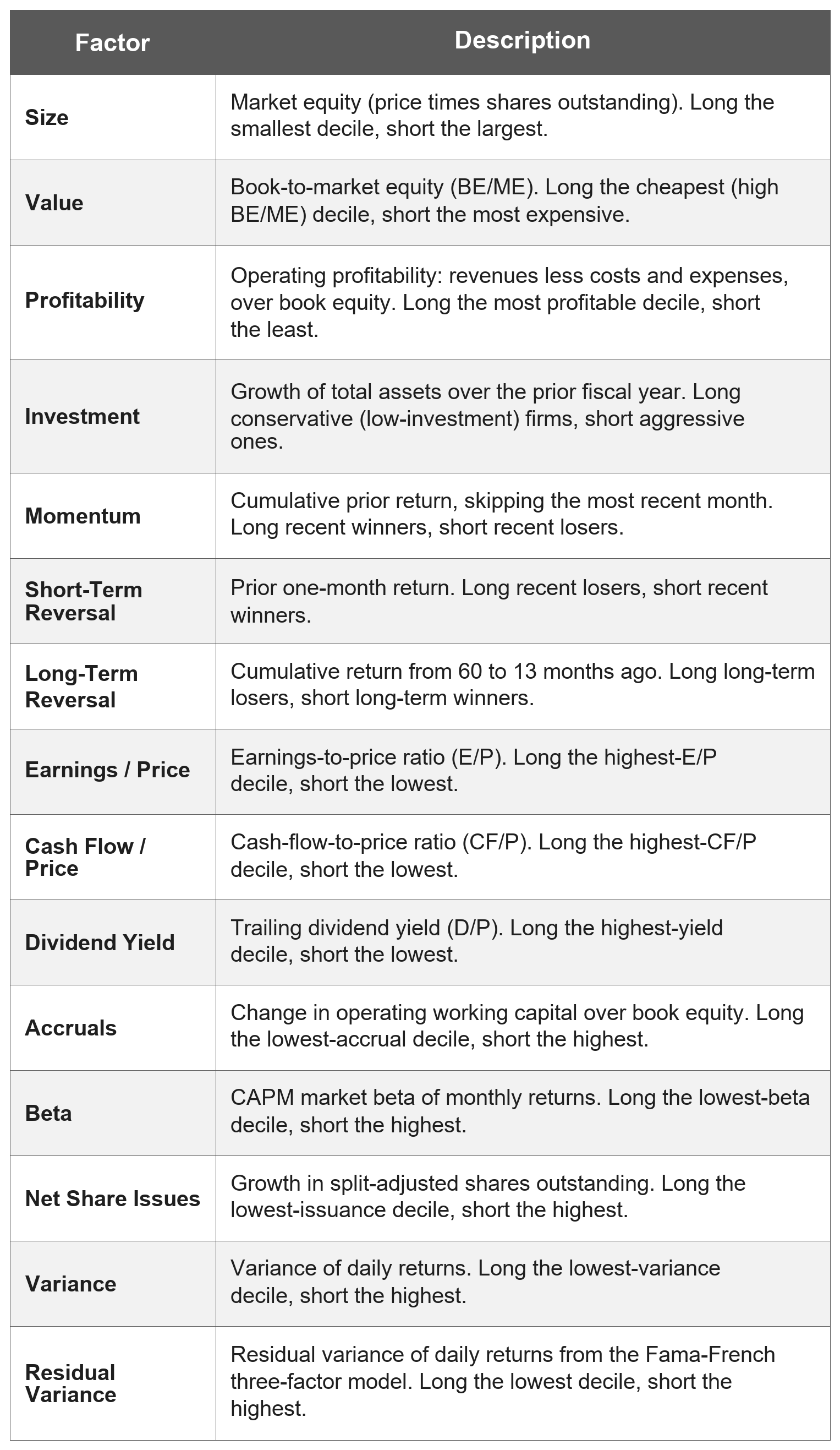
Our study relies on monthly data and covers fifteen anomalies made available within the French Data Library for US markets. Full details are provided in the table below.
For all factors, both the long and short legs are sized to target 20% annualized volatility, using a 12-month rolling standard deviation of log monthly returns as our volatility proxy. Formally, for each month t:
The monthly return of each factor portfolio is then computed as:
Cross-Sectional Momentum
The Panjabi-Bordigoni-Buchanan article provides a useful starting point for defining our cross-sectional signal:
“…we can adopt a cross-sectional, market-neutral approach. To put it another way, rather than applying univariate time-series models, we can apply a multi-variate framework based on the relative momentum of the sectors. This means being long those sectors exhibiting the strongest past performance and short the weakest, creating a portfolio with ex-ante market neutrality.”
While the exact formulation behind their relative-strength measure remains proprietary, we can start by simply defining each factor’s momentum (Mi,t) as its return over the prior 12 months:
A useful feature of constructing factors from volatility-scaled legs is that their trailing returns are directly comparable, without requiring further normalization. Cross-sectional sorts are most meaningful when applied to like-for-like portfolios: ranking raw returns across portfolios with very different risk levels could otherwise distort the ordering. Because all fifteen factors use the same volatility target for each leg, this issue is materially reduced.
Results
Our simulation starts in January 1985 and runs through May 2026, a span we split into two 20-year samples: 1985-2005 and 2006-2026.
We begin by testing whether the factor-momentum rank observed at each month-end (t) contains information about returns in the following month (t+1). For each rank, we calculate the average next-month returns separately by time sample and weighting scheme (equal- and value-weighted decile portfolios). The chart below reports the results.
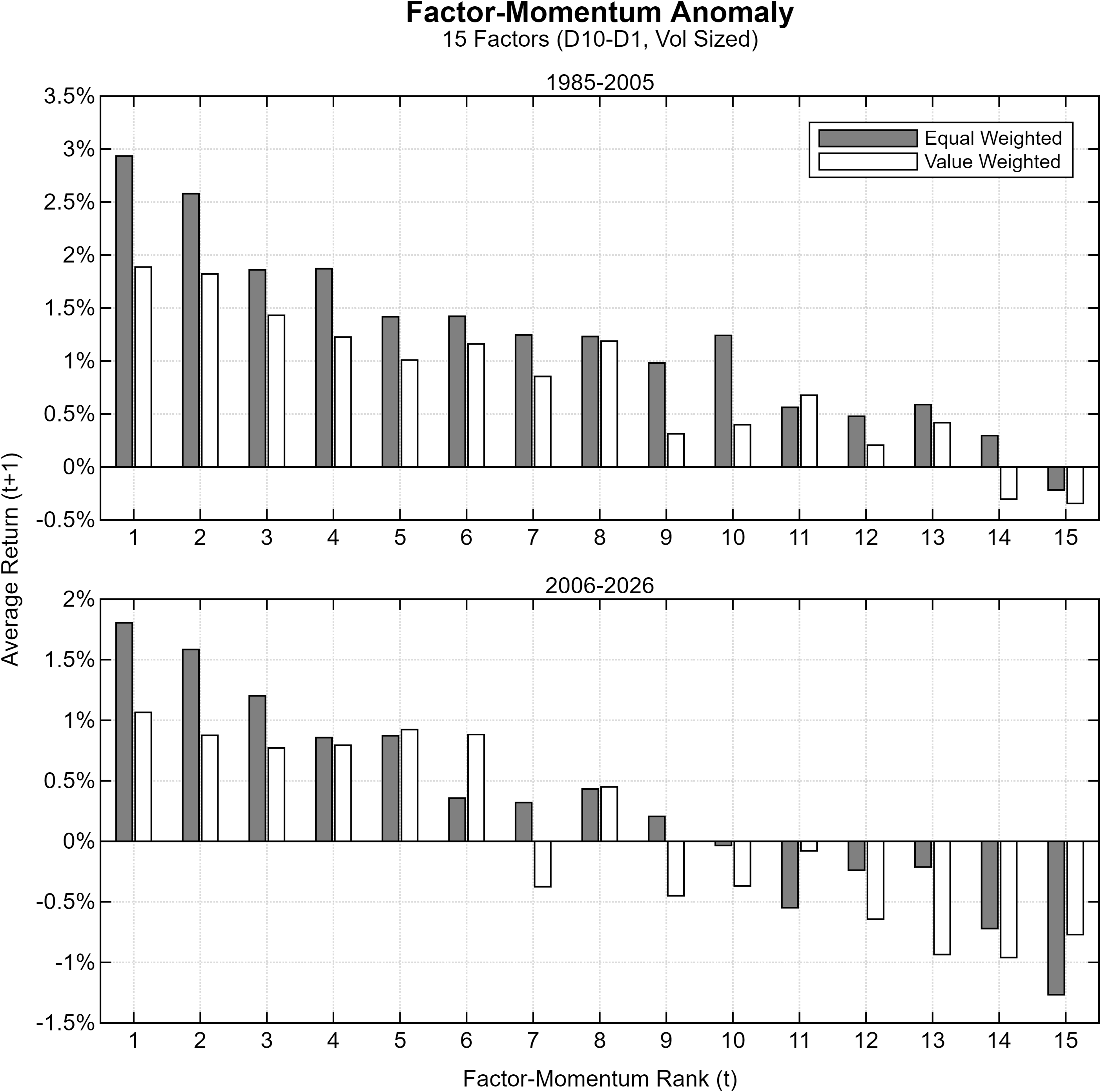
The results appear encouraging: the average next-month returns decline steadily as ranks move from 1 (the strongest relative-strength factor) to 15 (the weakest). The relationship is not perfectly monotone (with a few middle-ranks step out of line) but the overall slope is rather clear, and it shows up for both the equal-weighted (EW) and the value-weighted (VW) constructions, in both 20-year samples.
To translate this rank-return relationship into a simple strategy, each month we buy the three strongest factor portfolios and sell short the three weakest, based on their prior 12-month returns. The nine middle-ranked factors receive no allocation.
The chart below compares this strategy against a “passive” benchmark that holds all fifteen (volatility-sized) factors in equal weights and rebalances monthly. Within the figure, rows separate the weighting scheme (EW above, VW below) and columns split the two 20-year samples.
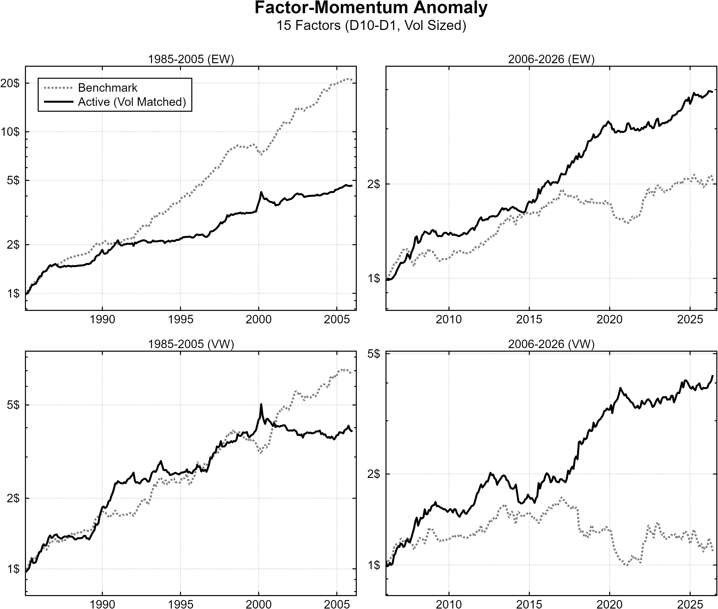
Notably, before 2006, the active portfolios fail to outperform the unconditional benchmark. We believe this result is largely a consequence of evaluating the strategy over the original factor-discovery period. By construction, the factors documented in the academic literature were identified precisely because they delivered positive returns during this sample. As a result, even the relatively weaker factors assigned to the short side often continued to exhibit positive returns.
This creates a structural headwind for the long-short implementation: the short leg is systematically positioned against factors that still possess positive in-sample drift. By contrast, the benchmark remains long every factor and therefore captures the full benefit of this broad-based appreciation.
After 2006, the picture changes materially. This period is arguably the more informative sample because many canonical factors had entered their genuine out-of-sample, post-publication phase. Published anomalies often experience substantial performance decay thereafter, whether because of arbitrage, changing market conditions, or the possibility that some original findings reflected data-mining artifacts.
In such an environment, an unconditional allocation across all factors becomes less compelling. The cross-sectional momentum strategy instead reallocates capital toward factors that continue to display relative strength and takes short exposure to those whose premia have faded. As a result, the active portfolios continue compounding, while the benchmark advances much more slowly or, in the value-weighted case, scarcely at all.
The same conclusion emerges from risk-adjusted returns. Sharpe ratios are recomputed within each 20-year sample for both the equal-weighted and value-weighted portfolios and are shown below.
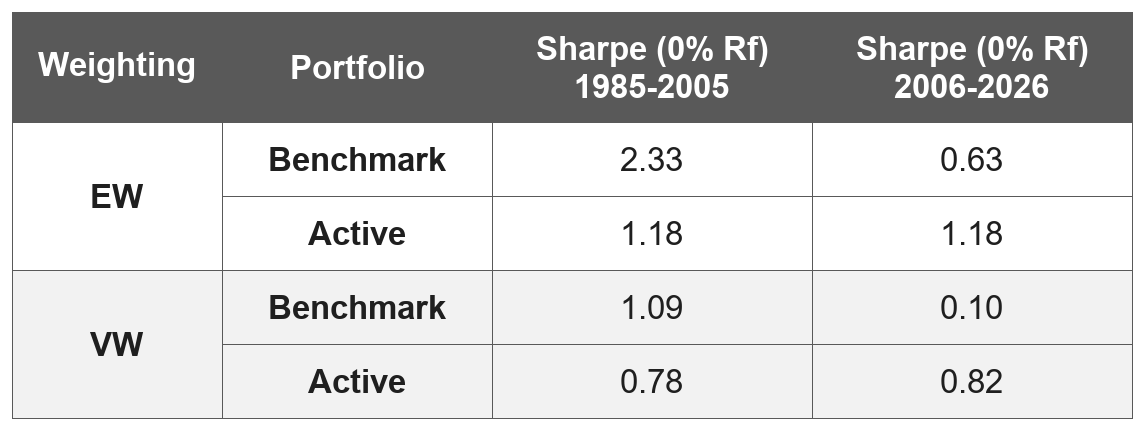
Over 1985–2005, the equal-weighted benchmark produced a remarkable Sharpe ratio of 2.33, compared with 1.18 for the active portfolio. Under value weighting, the corresponding figures were 1.09 and 0.78. Over 2006–2026, however, the pattern reverses: the benchmark falls to 0.63 under equal weighting and just 0.10 under value weighting, while the active portfolio remains at 1.18 in the equal-weighted case and improves to 0.82 in the value-weighted case.
How About Time-Series Momentum?
Having found robust evidence of cross-sectional momentum effects, we additionally check for time-series (i.e. trend) effects. Here the timing signal (s) no longer depends on the monthly cross-sectional sort: each factor (i) is simply traded long or short according to the sign of the 12-month momentum feature calculated earlier. Formally:
The simulated results are presented below, using the same benchmark described earlier for comparison.
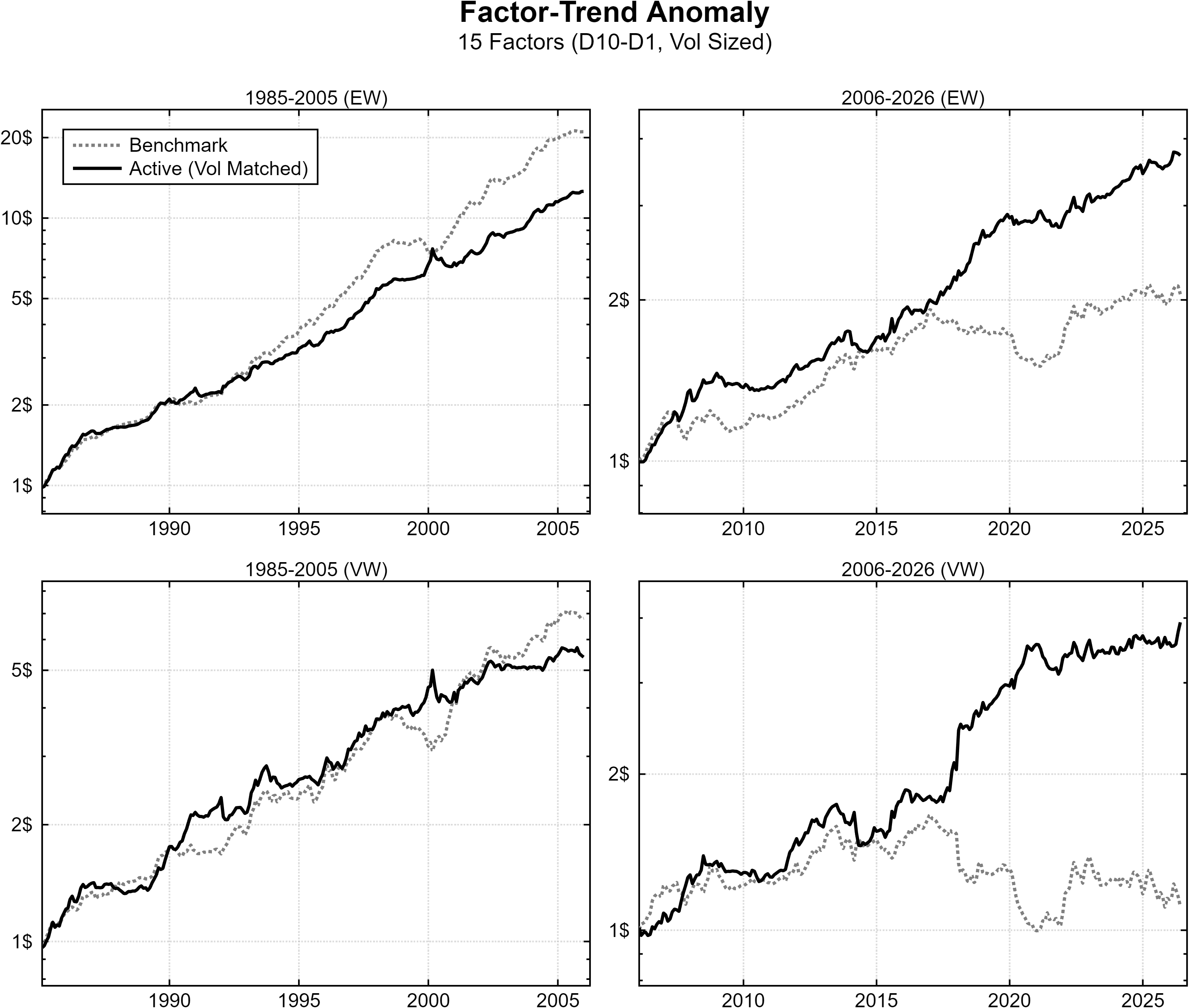
The time-series signals tell a similar story. The active factor portfolio trails the always-long D10-minus-D1 basket during the first sample but navigates the post-2006 environment much more effectively. As before, the result holds under both equal-weighted and value-weighted factor constructions.
Practical Implications
The portfolios presented throughout this article should primarily be viewed as academic building blocks rather than directly tradable investment strategies. Nevertheless, we believe the underlying findings are highly relevant for systematic investors seeking practical ways to dynamically allocate capital across equity factor premia.
In practice, however, implementing these strategies is far from straightforward. Academic factor portfolios require trading and, in particular, shorting hundreds of individual stocks. In reality, many names may not be available to borrow, and managing them introduces significant scalability and execution challenges.
Our follow-up article explores a framework for translating these rotational factor-momentum models into more investable portfolios: a natural next read if you're interested in the practical implementation of these ideas. Click the banner below to subscribe and receive it upon publication.

Conclusion
Overall, our results confirm the findings of Panjabi, Bordigoni, and Buchanan (2026) with a meaningful degree of robustness.
Across our factor universe, both cross-sectional and time-series momentum effects appear in each of the two 20-year samples and under both equal-weighted and value-weighted decile constructions.
However, the most interesting finding is not that factor momentum exists, but when active factor selection becomes most valuable.
During the original discovery period, nearly all documented factors exhibited positive drift by construction. In that environment, a long-short allocation faces an inherent disadvantage because its short leg is positioned against factors that were (obviously) producing positive returns. An unconditional, always-long allocation can therefore be difficult to beat.
Once these factors enter their post-publication period, the economics change. Some premia weaken, some become crowded or arbitraged away, and others may reveal themselves to have been partly sample-specific. In that setting, unconditional exposure becomes substantially less attractive, while momentum-based allocation offers a systematic way to bet on factors that continue to work and against those whose premia have weakened or reversed.
Viewed against the broader “factor zoo,” this distinction is important. The term, popularized by John Cochrane, describes the proliferation of empirical factors beyond the Capital Asset Pricing Model (CAPM). By some estimates, several hundred factors have now been published, raising persistent concerns about data mining and weak out-of-sample performance (Harvey, Liu, and Zhu, 2016).
In such a landscape, momentum-based approaches (whether cross-sectional or time-series) for factor investing deserve further study not merely as standalone anomalies, but as practical allocation tools for navigating a large and evolving universe of equity styles.
If you found this article useful, feel free to leave a comment or contact us by direct message or at info@concretumgroup.com.

Disclaimer
This publication is provided by Concretum Group for informational, educational, and research purposes only. It does not constitute investment, financial, legal, or tax advice, nor a recommendation to buy or sell any security, instrument, strategy, or investment product. All investments involve risk, including possible loss of principal. Past performance, backtested performance, and historical analysis are not reliable indicators of future results. Readers should conduct their own research and consult qualified professionals before making investment decisions.
Full disclaimer: https://concretumgroup.com/disclaimer/