


We wanted to see whether a long-only, rules based algorithm applied to US industries could remain profitable over a full century. Our paper written with Gary Antonacci, A Century of Profitable Industry Trends, answers exactly that. Using Kenneth French’s industry data from 1926 to 2024, the strategy delivers 18.2% compounded per year, with 12.6% volatility and a Sharpe ratio of 1.39.
For comparison, a passive market investment over the same period returns 9.7% per year, with 17.1% volatility and a Sharpe ratio of 0.63. Maximum drawdown falls from 84% to 33%, while annualized alpha is 10.9%.
In this article, we will go over the theory behind the paper and then show, step by step, how to replicate the results using our backtesting notebook. You just need to run the notebook, and the results will be generated for you.
You can also edit the parameters as you see fit and run the backtest again to explore different ideas and variations of the strategy.
This paper was awarded the 2025 Charles H. Dow Award by the CMT Association.
What’s the theory behind the algorithm?
The papers we reviewed from academia focus on monthly, cross sectional momentum, where the latest winners are bought relative to the rest of the universe, while the losers are shorted.
In this paper however, were not doing relative ranking, were trend following.
Each industry is its own price history. If the industry is not in an uptrend, the weight will be zero, and nothing will be shorted. The idle cash is invested in 1-month Treasury bills.
We did this to replicate discretionary and CTA-style trading, where you wait for a trend to appear, get in, and get out when the trend is no longer there. It also keeps exposure to the long-term equity risk premium.
The algorithm is built around three basic blocks:
Entry
Sizing
Exit
The Entry: Upper Band
We computed the breakout indicators, including the Keltner and Donchian Channels, after reconstructing the price series from the daily total returns.
In this case both indicators include a noise region. Price can oscillate inside the channel without forcing a trade.

Keltner Channels
In modern use, the center line is an exponential moving average and the width is a multiple of Average True Range:
Our data source, the Kenneth R. French - Data Library, provides closing prices only. Since there are no high or low prices, we cannot compute the ATR in the usual way.
Looking at the last 20 years of OHLC data, the 20-day ATR is about 1.4 times the 20-day average of absolute daily price changes, and that ratio is fairly stable.
So we assume:
Where n = 20 and k = 2 for the upper band; n = 40 and k = 2 for the lower band. The slower lower band is intentional. It creates an economic bias toward staying long through moderate pullbacks.
Donchian Channels
The highest high and lowest low over a lookback. With close-only data, that is the rolling max and min of close:
Where 20 days up, 40 days down. Same asymmetry as Keltner.
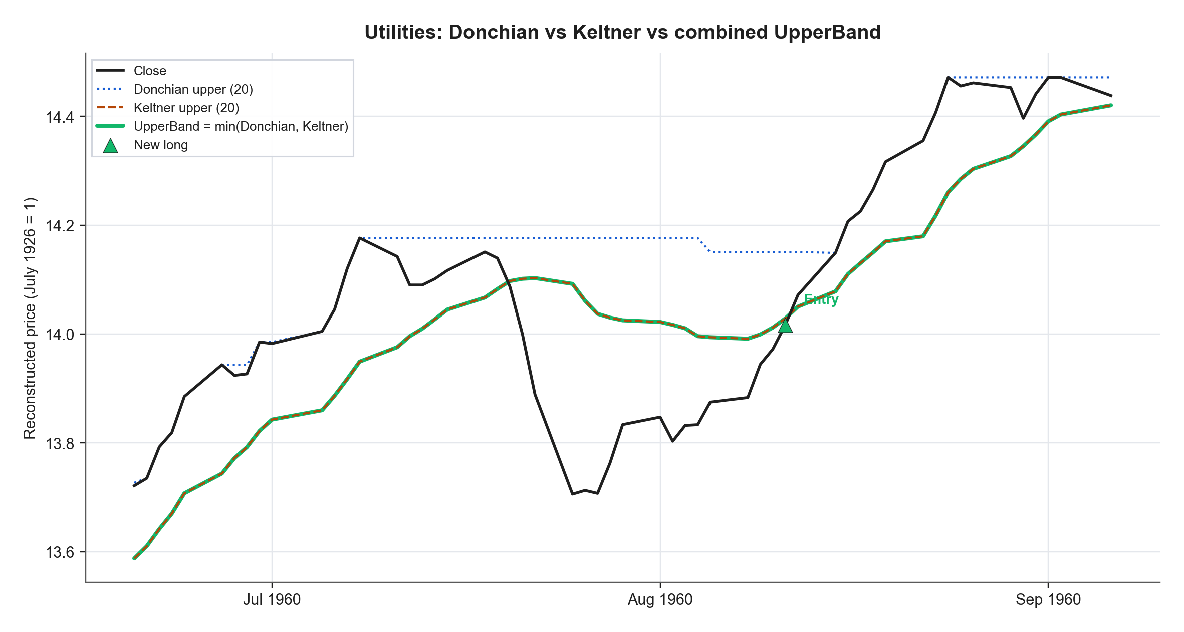
Combined entry rule
The algorithm does not wait for both indicators to agree. It enters when price shows strength on at least one of them. Realistically, this means using the tighter of the two upper bands:
A long is opened when
In the paper, about 69% of entries come from the Donchian upper band and 31% from Keltner.
The Sizing: Equal Volatility Contribution, Then Constraints
When an industry is in an uptrend, we scale the position by volatility so that each active industry contributes roughly the same amount of risk. This follows the practical approach used in CTA-style trading.
We set the portfolio volatility target for each industry at 1.5% / N, where N is the number of industries in the universe. The position weight is then based on inverse recent volatility. If an industry is not in an uptrend, its weight is simply zero.
There are also two constraints. Total exposure cannot exceed 200%, so if it does, all active positions are scaled down proportionally. In the notebook, we also cap any single industry at 20%. You can adjust this parameter as you see fit to simulate different outcomes.
Positions are marked and rebalanced daily. Idle cash earns the T-bill return, and any exposure above 100% is treated as borrowed at the same T-bill rate.
For the century-long French backtest, we do not include commissions or slippage. Market microstructure in the 1930s was obviously very different from 2024. Cost sensitivity is covered separately in the paper’s ETF section.
We saw about 99.5% of days are sized by the volatility target, while the leverage cap only binds on about 0.5% of days. Gross exposure can still vary a lot, with the 1-year average notional ranging from about 18% in 1933 to 195% in 1955. Beta tends to rise in strong markets and fall in weak ones.
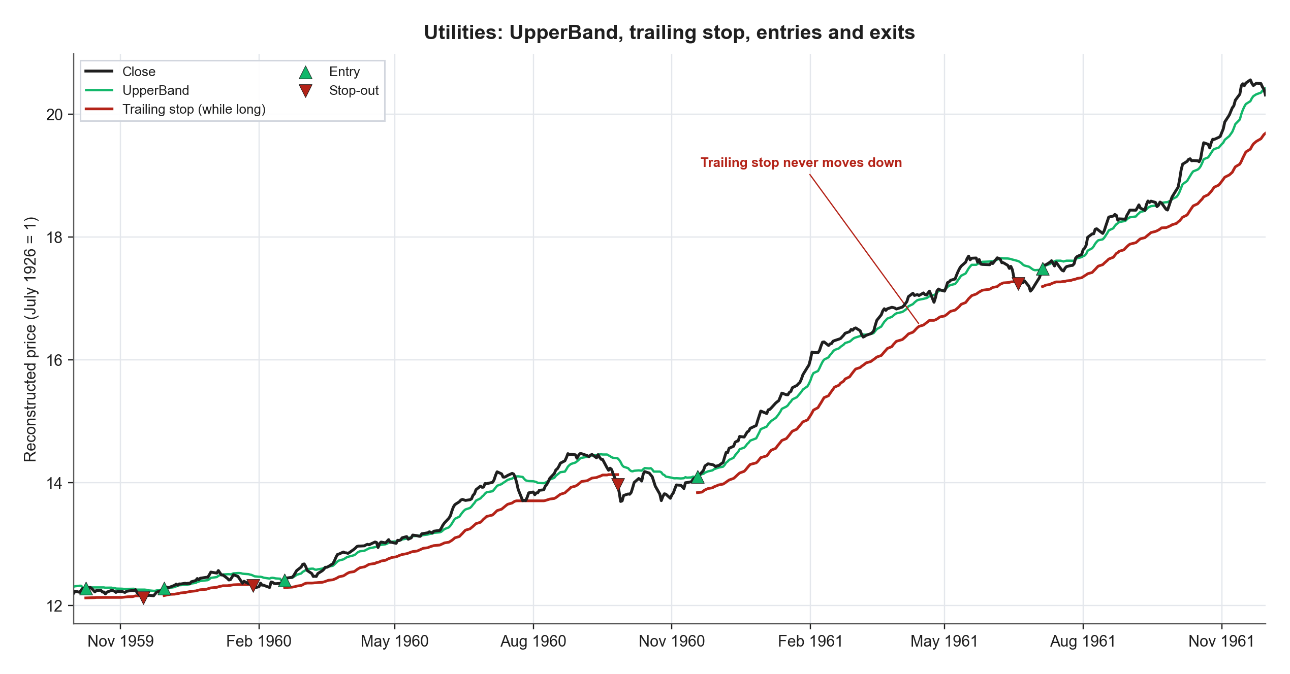
The Exit: A Trailing Stop That Never Eases
The stop is built from the same two indicators, using the more conservative lower band:
Trend followers do not give back stop protection after a trend has worked. The live trailing stop is ratcheted:
The position stays on as long as price holds above that trailing stop. It is closed when price closes through it. The stop is never moved down.
Most exits (85% in the paper) are Keltner lower-band stops.
What the Century-Long Backtest Shows
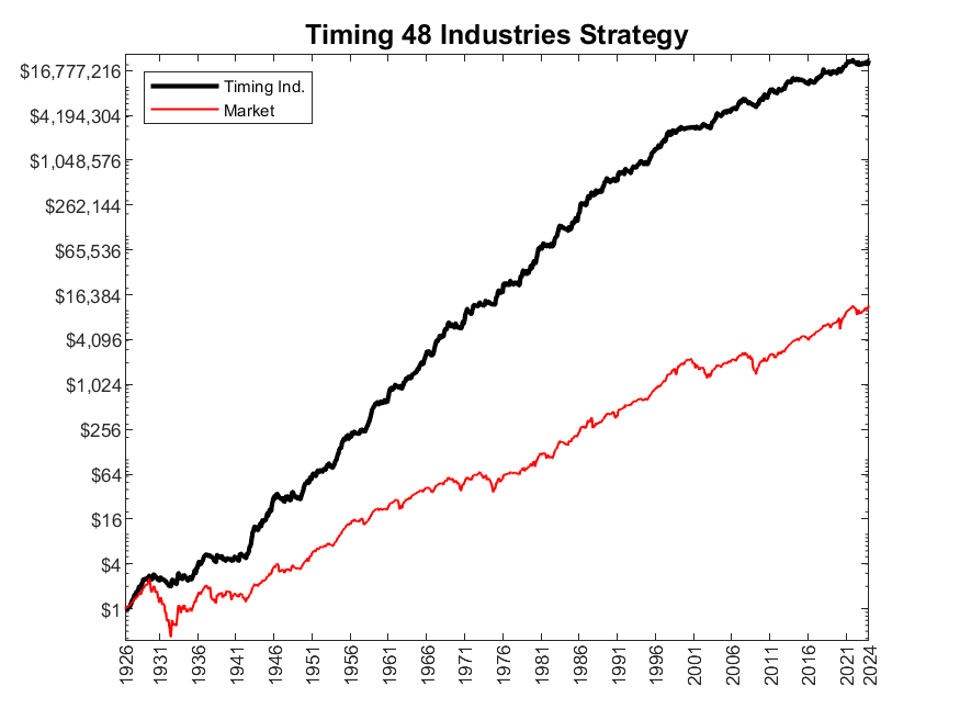
From July 1926 to March 2024, $1 in the market grows to about $16,000. $1 in the Timing Industry portfolio grows to more than $25 million. The path is not a straight line, but the drawdowns are shallower and shorter than buy-and-hold.
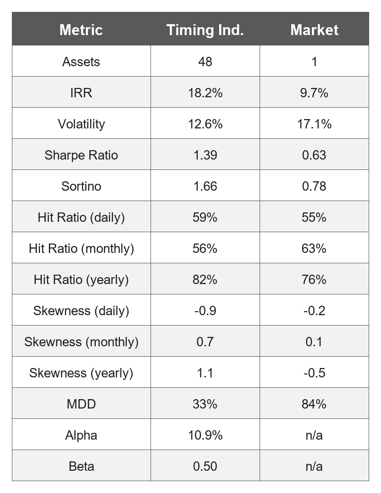
We saw that daily skew is more negative than the market, while monthly and yearly skew turn positive. The pattern is typical for trend following. You get a smooth move higher, followed by a sharp end to the trend. A few bad days can give back recent gains without wiping out the longer-term profit.
If we look at yearly returns, participation is above 1 in positive years and about 0.31 in negative years. The worst calendar year for the timing book is about −15%.
We applied the same rules to 31 State Street sector ETFs from 2005 to 2024, including commissions and slippage. The ETF results stay close to the French industry results and remain profitable under relatively high cost assumptions. That implementation is in the paper, not this notebook.
French’s files are still updated, so if you run the notebook today, the sample will extend past March 2024. Because of this, the headline numbers will not match the paper exactly.
How to Run the Backtest
You can simply click Run all, and everything will be taken care of.
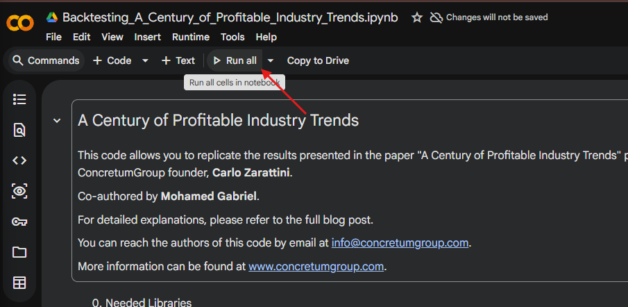
You can also edit the parameters as you see fit, then run the second cell to see the updated results.
user_params = [
    {
        "UP_DAY": 20,
        "DOWN_DAY": 40,
        "ADR_VOL_ADJ": 1.4,
        "KELT_MULT": 2.8,
        "AUM_0": 1,
        "invest_cash": "YES",
        "target_vol": 0.02,
        "max_leverage": 2,
        "max_not_trade": 0.20,
    },
]
This notebook runs entirely in the cloud, so there is nothing to download. Simply click Run All, then adjust the parameters to explore different results.
If you found this article useful, feel free to leave a comment or contact us by direct message or at info@concretumgroup.com.

Research Transparency Statement
Every research idea, hypothesis, methodology, dataset, code, backtest, analysis, and conclusion presented in this article was independently developed by the Concretum Group research team. Artificial intelligence tools were used as productivity assistants to support the preparation of the final article, including language refinement, grammatical review, and, where appropriate, the generation of visual elements such as tables and figures. All research decisions, analyses, interpretations, and conclusions remain entirely those of the authors.
Disclaimer
This publication is provided by Concretum Group for informational, educational, and research purposes only. It does not constitute investment, financial, legal, or tax advice: it is not a recommendation to buy or sell any security, instrument or investment product. All investments involve risk, including possible loss of capital. Past performance, backtested performance, and historical analysis are not reliable indicators of future results. Readers should conduct their own research and consult with professionals before making investment decisions. Click here for the full disclaimer.
the 20 up, 40 down asymmetry is the detail i'd point people at. a slower exit than entry keeps you in through the pullbacks, and the stop that never eases does the rest. i run a channel breakout on futures with the same only-tightens rule. did you test how much of the 1.39 sharpe comes from the asymmetry versus a symmetric 20/20?
The notebook is a useful touch. Being able to rerun the test and change one assumption makes the result much easier to interrogate.