

Global Tactical Asset Allocation, Automated With Python and IBKR
Revisiting Meb Faber’s 2007 Classic, Updated Through 2025 and Built for Live Execution

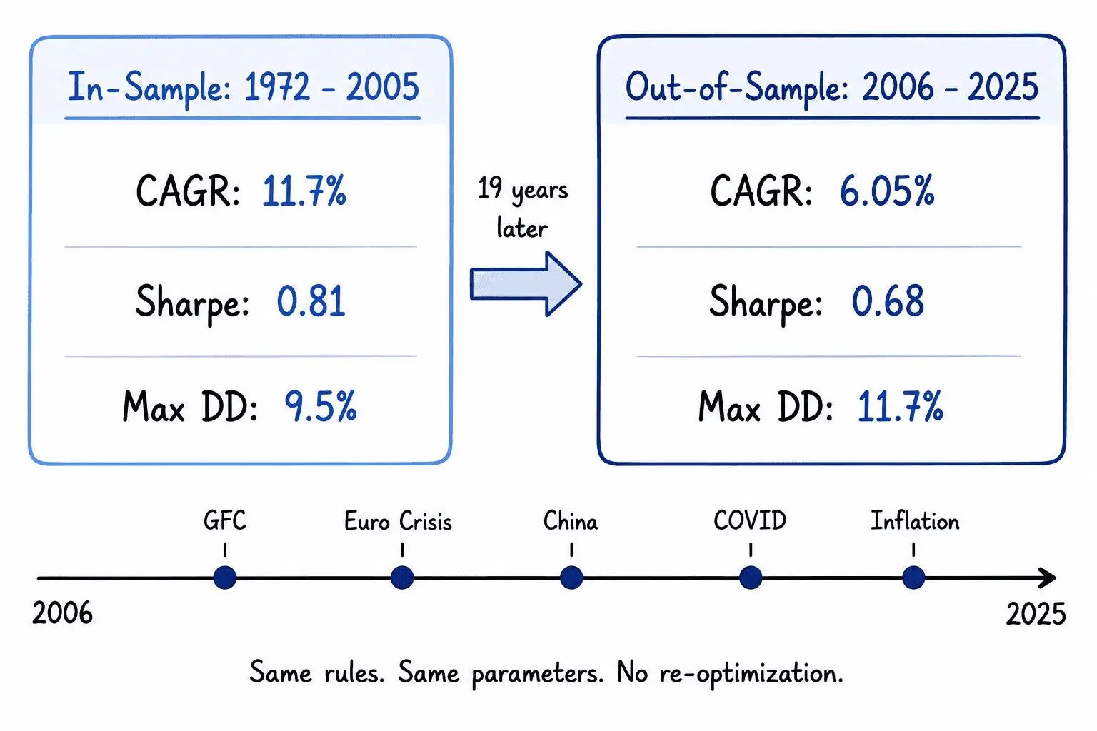
Meb Faber published A Quantitative Approach to Tactical Asset Allocation in 2007. It became one of the most influential investment research papers of the past two decades. The rules are simple: five asset classes, one trend signal per asset, monthly rebalancing. The original backtest ran from 1972 to 2005 and produced a Sharpe ratio of 0.81, a CAGR of 11.7%, and a maximum drawdown of 9.5%.
We wanted to know if it still works. So we ran it on the next 20 years of data, 2006 through March 2025, a period the strategy had no input in shaping. It does. Sharpe ratio of 0.68, CAGR of 6.05%, maximum drawdown of 11.7%, across the Global Financial Crisis, the COVID crash, and the 2022 inflation selloffs.
We published the full analysis in our paper Global Tactical Asset Allocation: Updated Results and Real-Market Implementation Using Python and IBKR, which is publicly available. We also built a Python notebook that automates the entire rebalancing process through Interactive Brokers.
This article covers the strategy in full: how it works, why a critical implementation detail can silently cost you more than 2% per year in CAGR, how to fix it, and how to run the whole thing automatically through a Jupyter notebook connected to a live broker account.
Note: Treat this as an educational starting point. Run your own tests. Validate the signals. Stress-test the execution before putting real capital at risk.
What Is Tactical Asset Allocation?
Most long-term investors pick a fixed allocation and hold it through everything. 60% stocks, 40% bonds. They rebalance once a year and ignore the noise in between. That’s strategic asset allocation (SAA). It is simple, transparent, and easy to implement, but it also assumes that the optimal portfolio today is likely to remain the optimal portfolio through bull markets, bear markets, inflation shocks, and financial crises.
Tactical asset allocation (TAA) works differently. Instead of holding fixed weights through every market environment, it adjusts exposure according to a predefined set of rules. Different tactical approaches use different signals. Some rely on economic data, valuations, or market sentiment. Others, like the strategy examined in this article, use price trends.
The idea is simple. When an asset is in an uptrend, it is held in the portfolio. When the trend deteriorates, the position is reduced or eliminated, with the proceeds typically moved to cash or short-term bonds.
The primary goal is not necessarily to maximize raw returns, but rather to improve the balance between return and risk by reducing exposure during unfavorable market environments. Investors who lose 50% need a 100% gain just to recover. Cutting that peak-to-trough loss in half changes the long-term compounding math dramatically.
The key constraint is that this has to be systematic. No human judgment, no market calls, no emotion. A fixed rule that runs the same way every time, regardless of what the news says.
The Original Faber Strategy
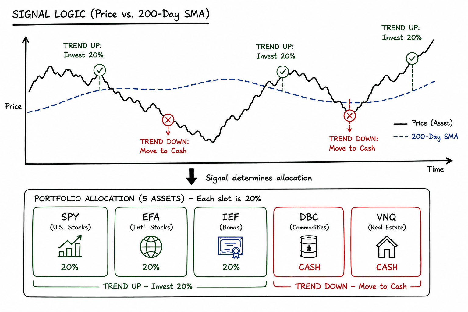
The strategy allocates capital across five total return indices, each representing a major asset class with genuine long-term return potential.
The five assets:

The signal rule: at the end of each month, compare the closing price of each asset to its 200-day simple moving average.
Price above the 200-day SMA: invest 20% in that asset
Price below the 200-day SMA: put that 20% into 90-day T-Bills instead
No bottom fishing. No macro view. No optimization. Each asset gets an equal 20% weight when it’s in an uptrend, and gets replaced with cash when it isn’t.
Over the 1972 to 2005 in-sample period, this produced a Sharpe ratio of 0.81, a CAGR of 11.7%, and a maximum drawdown of 9.5%. Note that the drawdown figure uses monthly observations, so the actual portfolio drawdown was likely somewhat deeper.
The paper made a big impact. The strategy is elegant, transparent, and grounded in a well-understood behavioral phenomenon: momentum. Assets that have been going up tend to keep going up, until they don’t.
The question is whether those results were the product of a genuine edge or a well-fit backtest.
Updated Results: 20 Years Out-of-Sample
We extended the analysis from where Faber left off: January 2006 through March 2025. No in-sample tuning. No parameter adjustment. The same 200-day SMA, the same five assets, the same monthly rebalancing at month-end.
The period included some brutal stress tests:
The Global Financial Crisis (2008-2009)
The European Sovereign Debt Crisis (2011)
The Taper Tantrum (2013)
The China Crisis (2015)
Volmageddon and the US-China Trade War (2018)
The COVID-19 pandemic (2020)
The inflation-driven selloffs of 2022
Despite all of it, the strategy held up.
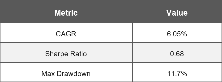
Returns came in below the in-sample period, which is expected. Strategies rarely perform as well out-of-sample as they do on the data they were designed on. But a Sharpe of 0.68 with an 11.7% maximum drawdown, earned through two decades of genuinely difficult markets, is a strong result for something this simple.
The Hidden Problem: Rebalance Timing Luck
Here’s something most backtests don’t address.
The original strategy rebalances at month-end. But there is no particular reason why the last trading day of the month should be privileged over the 10th, the 15th, or the 20th trading day. These are all reasonable implementation choices for the same underlying strategy.
The question is not which day is “correct”. The question is how much the results depend on that choice. If two investors follow identical rules but rebalance on different days of the month, how different can their outcomes become?
To answer that question, we ran 21 separate simulations of the same Global Tactical Asset Allocation (GTAA) strategy. Each one rebalanced on a different trading day of the month: from n=0 (last trading day) all the way to n=20 (the 20th trading day). Same strategy, same signals, same assets. Only the rebalancing day differed.
The spread was striking.
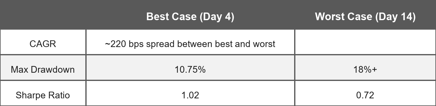
Nearly 220 basis points of CAGR difference between the best and worst rebalancing day. That's not a rounding error. That's the difference between a strong result and a mediocre one, and it has nothing to do with skill or alpha. It's pure timing luck.
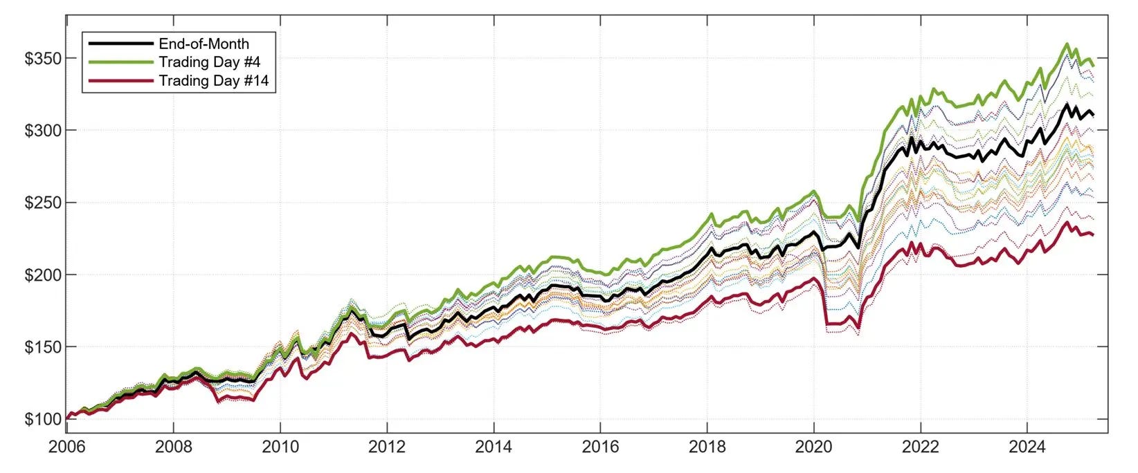
This is called rebalance timing luck. It is a well-known issue among asset managers and wealth management practitioners, yet it is rarely quantified in backtests. When signals are binary and rebalancing is infrequent, the exact moment you check the price relative to the moving average can determine whether you catch a trend early or miss it entirely.
The Fix: Tranched Weekly Rebalancing
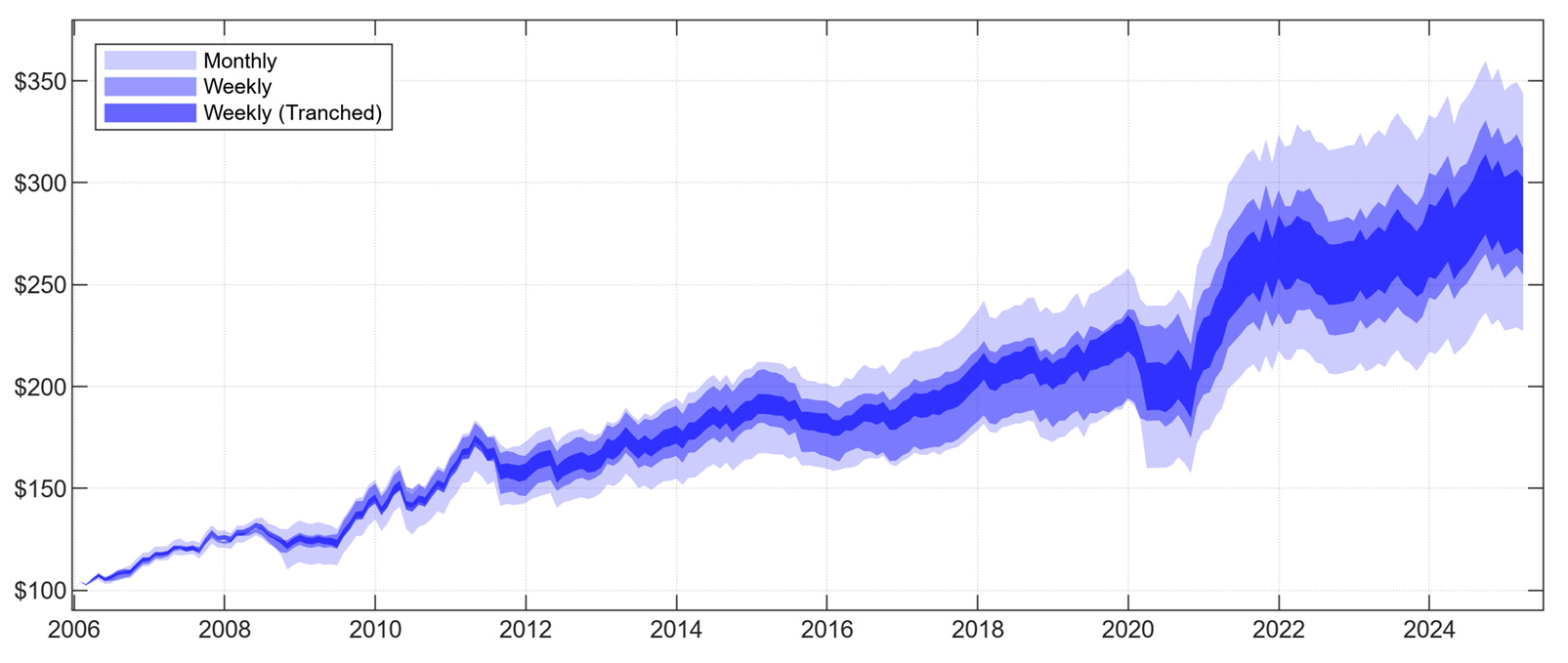
The simplest solution is to rebalance more often. If you check signals weekly instead of monthly, you’re averaging across more observations, and the impact of any single unlucky day is smaller.
We ran weekly simulations on each day of the week. The CAGR spread shrank from 220 basis points to under 130 (and under 50 if you exclude Monday, which consistently underperformed).
But higher frequency rebalancing introduces a different problem: whipsaw.
When a signal flips from 1 to 0 and back again over several consecutive weeks, a weekly rebalancer will enter and exit the same position multiple times. A monthly rebalancer would have never moved. Each unnecessary round-trip costs transaction fees and can generate losses from adverse short-term price moves.
The faster you trade, the more exposed you are to noise.
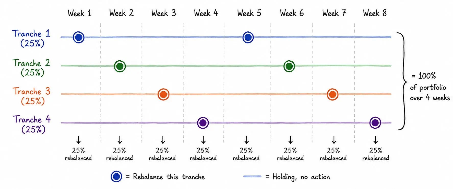
To get the stability of monthly rebalancing and the timing benefits of weekly execution, we propose a tranched approach.
The idea: split the portfolio into four equal sub-portfolios, each rebalanced on a staggered four-week cycle. You still rebalance weekly, but only one quarter of the portfolio moves at a time. Week 1, tranche 1 rebalances. Week 2, tranche 2. And so on.
The practical impact:
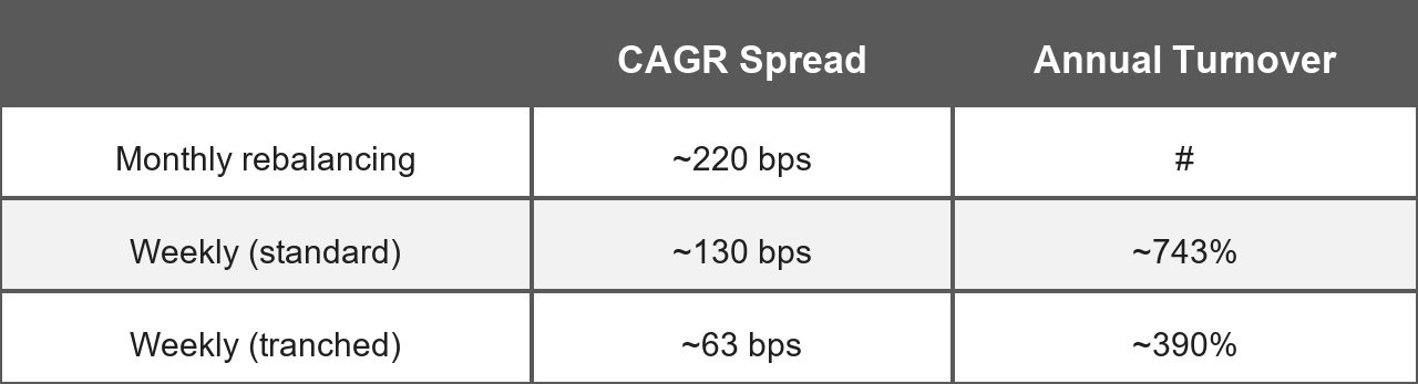
The outcome dispersion drops to 63 basis points. Annual turnover falls by nearly half. At 10 basis points of transaction costs per trade, that turnover reduction alone saves around 35 basis points of CAGR per year. Not transformative, but real, and it compounds.
One practical note on account size. With four tranches, each individual trade represents roughly 5% of the portfolio (25% of the portfolio, split across five assets). On smaller accounts, that can mean trade sizes too small to execute cleanly, especially if fractional shares aren't available or minimum commissions eat into the order. If tranche sizes get impractical, the simpler monthly approach is the right choice.
Signal Lag and Transaction Costs
Once the rebalancing structure is set, the next step is making the backtest honest about real-world friction.
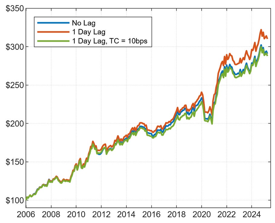
We took the Wednesday-tranched portfolio and added two elements. First, a one-day execution lag: signals are computed from Tuesday’s closing prices, and trades execute at Wednesday’s close. This mirrors how the notebook works in practice. You download data, run the signal, prepare the order, and submit it the next day. Second, transaction costs of 10 basis points applied to every notional amount transacted.
Two findings worth noting.
The one-day lag slightly improved results. This runs counter to intuition but is what the data shows.
The transaction costs reduced performance by approximately 41 basis points per year. That’s a real cost, but it’s contained. SPY, EFA, IEF, DBC, and VNQ are among the most liquid ETFs in the world. The 10 bps assumption is conservative.
Automating It
The Python notebook handles the full rebalancing workflow: fetching data, generating signals, calculating trade sizes, and submitting orders to Interactive Brokers. It works for both the original monthly approach and the tranched weekly version.
The six ETFs used:
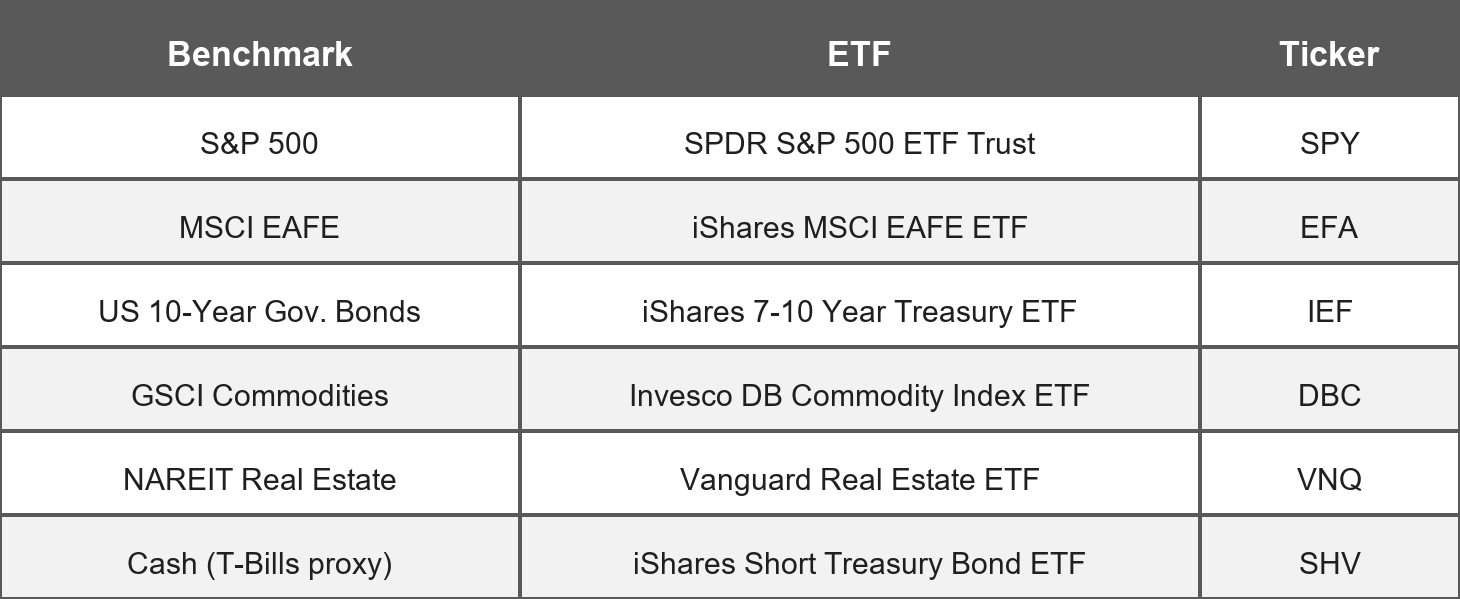
SHV serves as the cash proxy. Any capital not allocated to a trend-positive ETF gets invested in SHV. It always has a signal of 1 and can absorb any remaining allocation.
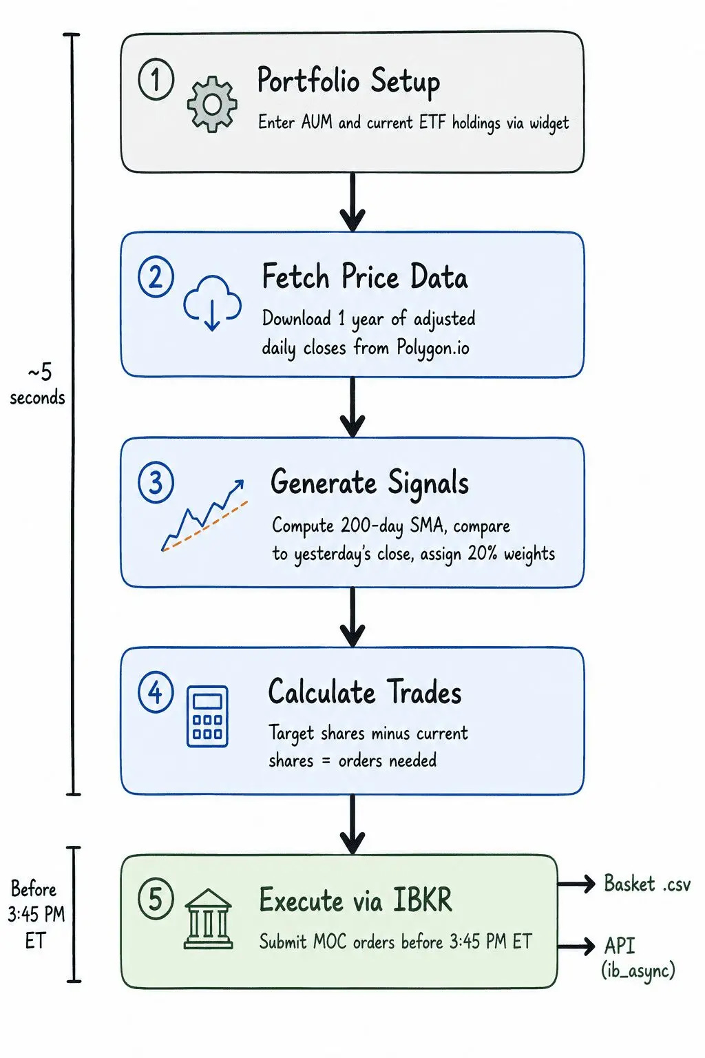
Step 1: Portfolio Setup
Before computing any signals, the notebook collects two inputs from the user through an interactive widget:
Total AUM allocated to the GTAA strategy
Current share counts for each of the six ETFs (only positions belonging to this strategy)
Step 2: Signal Generation
For each ETF except SHV, the notebook downloads one year of daily adjusted closing prices from Polygon.io and computes the 200-day SMA using yesterday's close as the most recent data point.
SMA_i = (1/200) x sum of P_i over the last 200 daysThe signal for each ETF is then:
Signal = 1  if yesterday's close > SMA
Signal = 0  otherwise
ETFs with a signal of 1 receive a 20% weight. ETFs with a signal of 0 receive nothing. Adjusted prices are used throughout to avoid false signals from dividends and stock splits.
Step 3: Rebalancing Logic
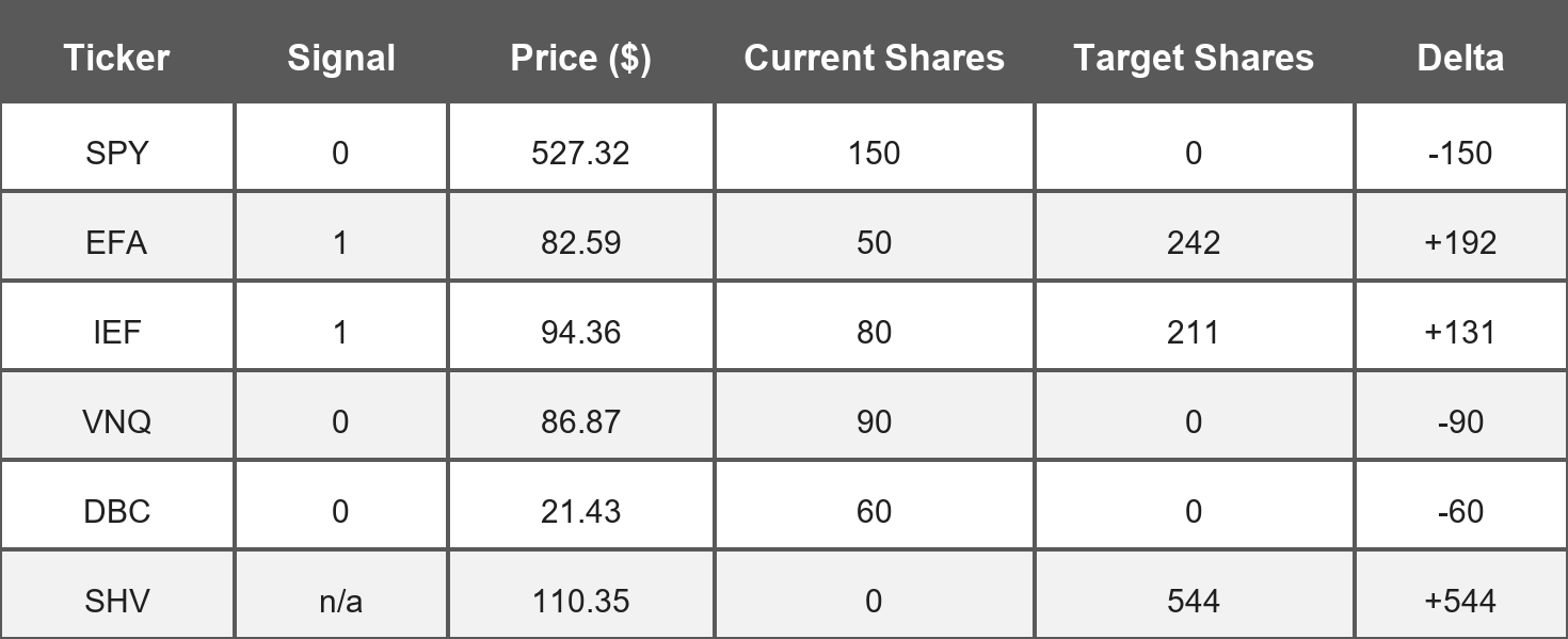
With signals and weights defined, the notebook computes what the portfolio should look like and calculates the trades needed to get there.
Target shares for each ETF:
Target Shares = (AUM x Weight) / Last PriceFor ETFs with a signal of 0, target shares are zero. The remaining unallocated capital goes into SHV.
Trade required per instrument:
Delta Shares = Target Shares - Current SharesThe output is a clean summary table:
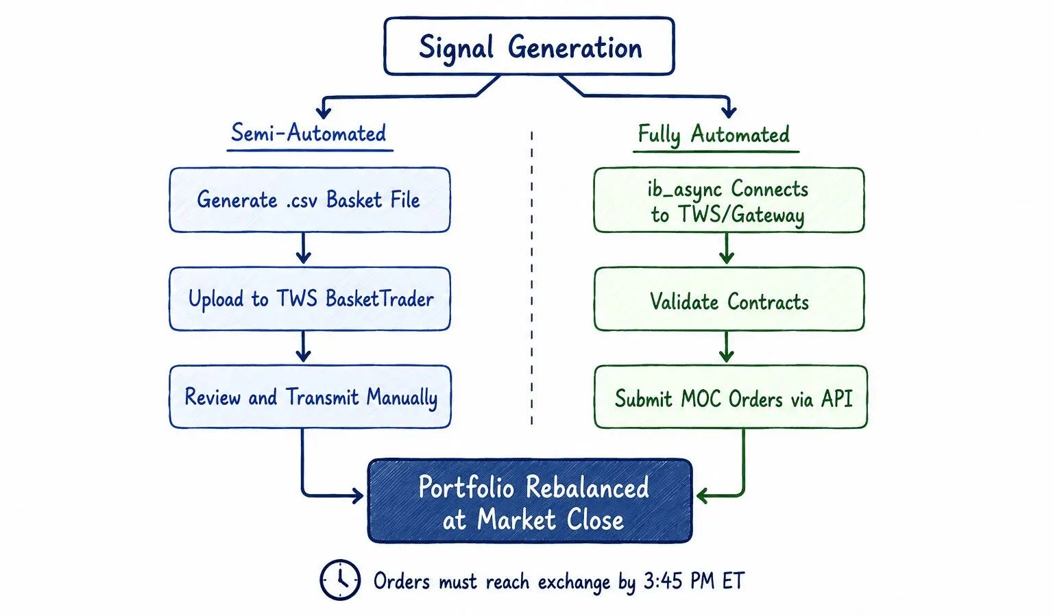
Step 4: Trade Execution via IBKR
The notebook supports two execution paths.
Semi-automated via TWS Basket File. For investors who want to review orders before anything gets sent to the exchange, the notebook generates a .csv file containing the full order list. Each row specifies the instrument, action (Buy or Sell), quantity, and order type (Market-On-Close). You load this file into Trader Workstation using the BasketTrader tool and submit it manually.
Fully automated via IBKR API. For fully hands-off execution, the notebook connects directly to TWS or IB Gateway through the ib_async Python package, validates each contract, and submits Market-On-Close (MOC) orders programmatically.
MOC orders must reach the exchange by 3:45 PM ET to guarantee execution at the official closing price. The notebook generates and submits orders immediately after computing signals, leaving a comfortable buffer.
After submission, the notebook confirms each order with its ticker, quantity, direction, and order ID. Every instruction sent from Python is mirrored inside Trader Workstation, so you can visually verify that what the code produced matches what the broker received.
Running It in Practice
Start with paper trading. Connect to IBKR’s paper trading account (port 7497) and run a full rebalancing cycle before touching real money. Verify that the signals look right, that the target positions make sense for your AUM, and that the orders go through cleanly. Don’t skip this step.
Enter your current holdings accurately. The notebook takes your share counts as manual input. If those numbers don’t match your actual positions, the trade calculations will be wrong. Before every run, pull your live positions from IBKR and type them in carefully.
Don’t miss the MOC deadline. Market-on-Close orders have to reach the exchange by 3:45 PM ET. The notebook submits right after computing the signal, which is fast, but don’t introduce delays between opening the notebook and running the execution cell.
Think about tranche size relative to your account. Each of the four tranches represents about 25% of your total allocation. On smaller accounts, the individual order sizes within each tranche can get very small, especially after dividing 25% across five ETFs. If fractional shares aren’t supported for a given ETF, or if minimum commissions start eating into your orders, the monthly version is the cleaner choice.
Check the output every time you run it. Connections to IBKR can drop. Data feeds can go stale. Orders can be rejected if the contract validation fails or if the submission comes in too late. The notebook logs everything to a CSV, so the full audit trail is always there. Check it.
Conclusion
Meb Faber published this strategy in 2007 and the core idea hasn’t changed: trend-follow five asset classes with a 200-day moving average, move to cash when the trend breaks. Eighteen years later, it still produces a Sharpe ratio of 0.68 on data it never saw.
What our paper adds is two things. First, a real-world stress test: 20 years of out-of-sample performance through the worst market crises of the modern era. Second, an honest look at a problem most practitioners ignore: rebalancing on a single fixed day each month introduces up to 220 basis points of CAGR variance that has nothing to do with the strategy itself. Tranched weekly rebalancing brings that down to 63 basis points and cuts annual turnover by nearly half.
The Python notebook makes this implementable. Data from Polygon.io, signal generation using the 200-day SMA, trade sizing, and direct execution through Interactive Brokers via MOC orders. Semi-automated or fully automated, your choice. The notebook is publicly available on Google Colab.
Trend-following is not a free lunch. It underperforms during choppy, mean-reverting markets. It can stay in cash for extended periods and miss rallies. And running any automated system live requires ongoing attention to execution quality, data integrity, and broker connectivity.
Start on paper trading. Study the signals. Build your own conviction in the logic before you put capital behind it.
If you found this article useful, feel free to leave a comment and reach out via direct message or email at info@concretumgroup.com for any questions.

Disclaimer
This publication is provided by Concretum Group for informational, educational, and research purposes only. It does not constitute investment, financial, legal, or tax advice, nor a recommendation to buy or sell any security, instrument, strategy, or investment product. All investments involve risk, including possible loss of principal. Past performance, backtested performance, and historical analysis are not reliable indicators of future results. Readers should conduct their own research and consult qualified professionals before making investment decisions.
Full disclaimer: https://concretumgroup.com/disclaimer/
Can you compare this strategy against the equal-weight monthly rebalanced portfolio of everything but SHV and a classic 60%/40% portfolio?