

The Complete Norgate Data Toolkit: Three Python Workflows Every Quant Researcher Needs
Building survivorship bias-free equities, point-in-time index membership, and a full futures database, all in Python.

Over the past several months, we published three standalone guides on building research-grade financial databases using Norgate Data and Python. Each one solves a different data construction problem that every systematic trader or quant researcher eventually runs into.
This article brings all three together in one place. We walk through what each workflow does, why it matters, and what it produces. The Jupyter notebooks are provided alongside this article so you can download them, configure the parameters, and run them directly.
Here is what we built:
Survivorship-Bias-Free U.S. Equity Database. The entire U.S. stock market, including delisted companies, enriched with sector classifications, company names, and index membership flags.
Point-in-Time Index Membership. Reconstructing which stocks actually belonged to an index (S&P 500, Nasdaq 100, Russell 3000) on any given date in history, with entry/exit dates and re-entry tracking.
Complete Futures Database Pipeline. Contract specifications, individual contract histories, continuous adjusted and unadjusted series, and volume decomposition across all futures markets.
Each section below explains the problem, describes the approach, and shows what you get at the end.
Part 1: Building a Survivorship-Bias-Free U.S. Equity Database
Why This Matters
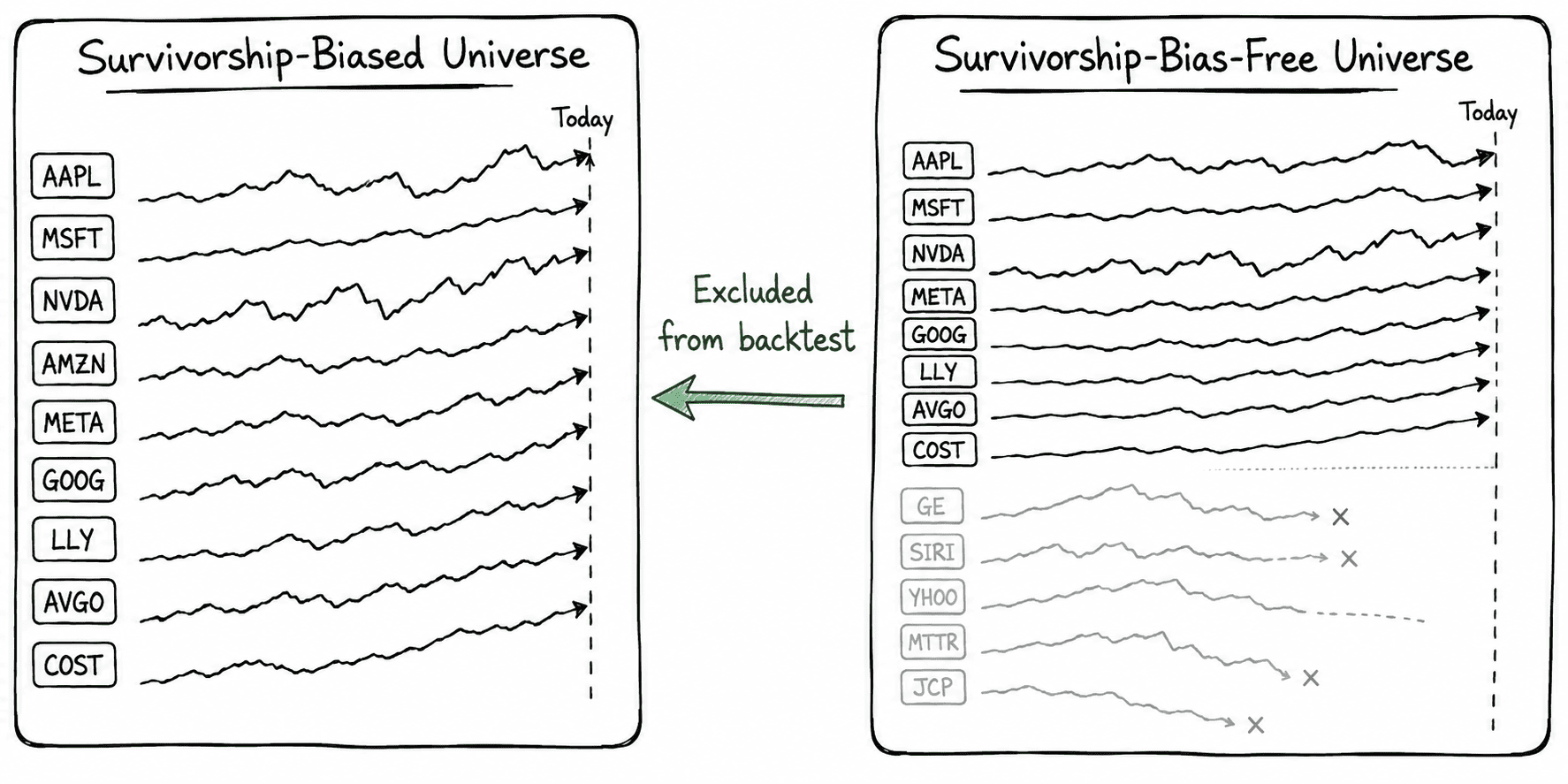
If you backtest a stock strategy using only companies that trade today, you are testing on the survivors. Companies that went bankrupt, got acquired, or were delisted for any reason are missing from your dataset. This is survivorship bias, and it consistently makes strategies look better than they actually were.
The fix is straightforward: include every company that ever traded, whether it is still active or not. Norgate Data maintains a complete archive of delisted U.S. equities alongside the active ones, and their Python API lets you pull both.
What the Notebook Does
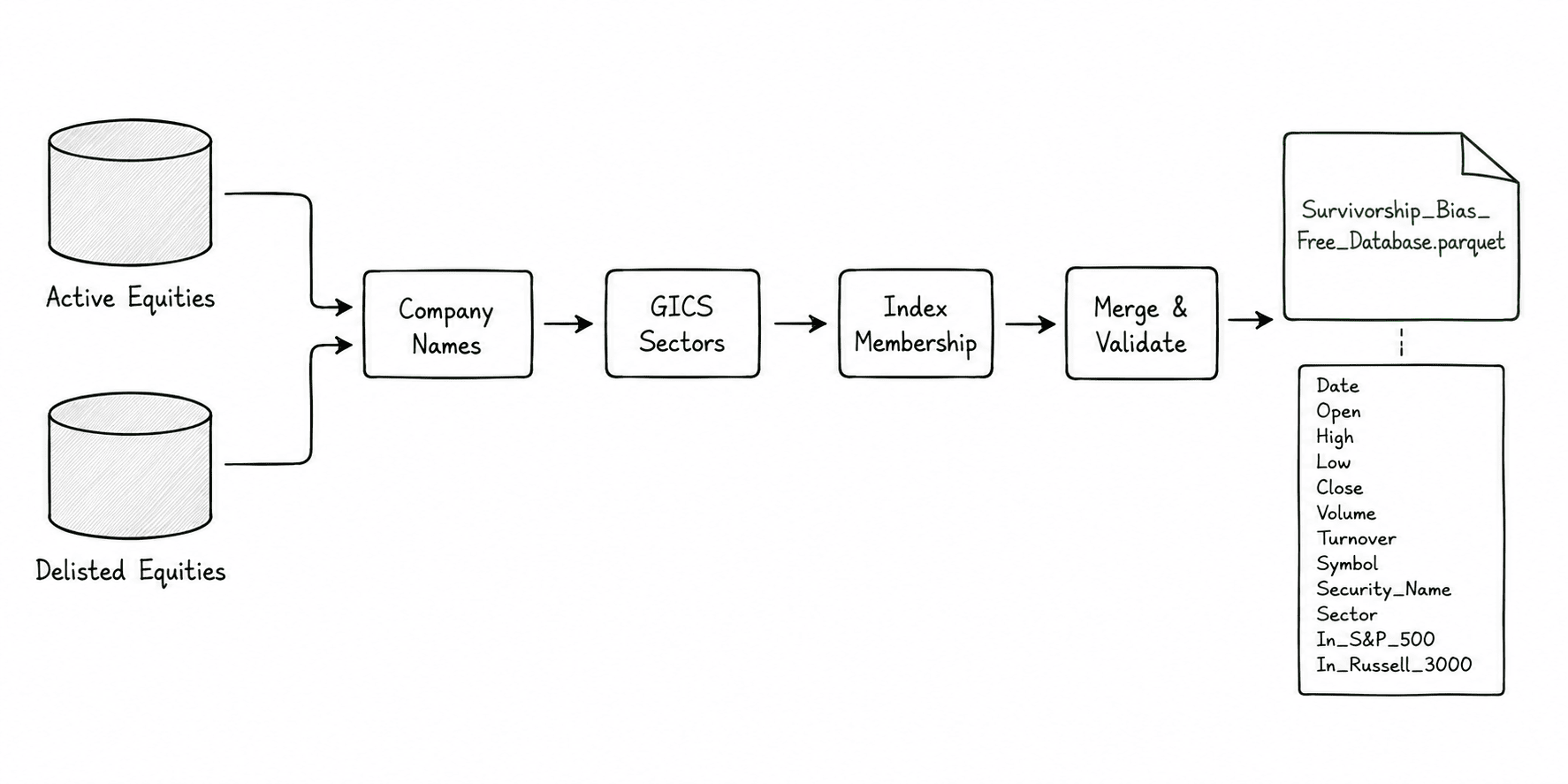
The workflow is a 12-step Jupyter notebook that starts small and scales up.
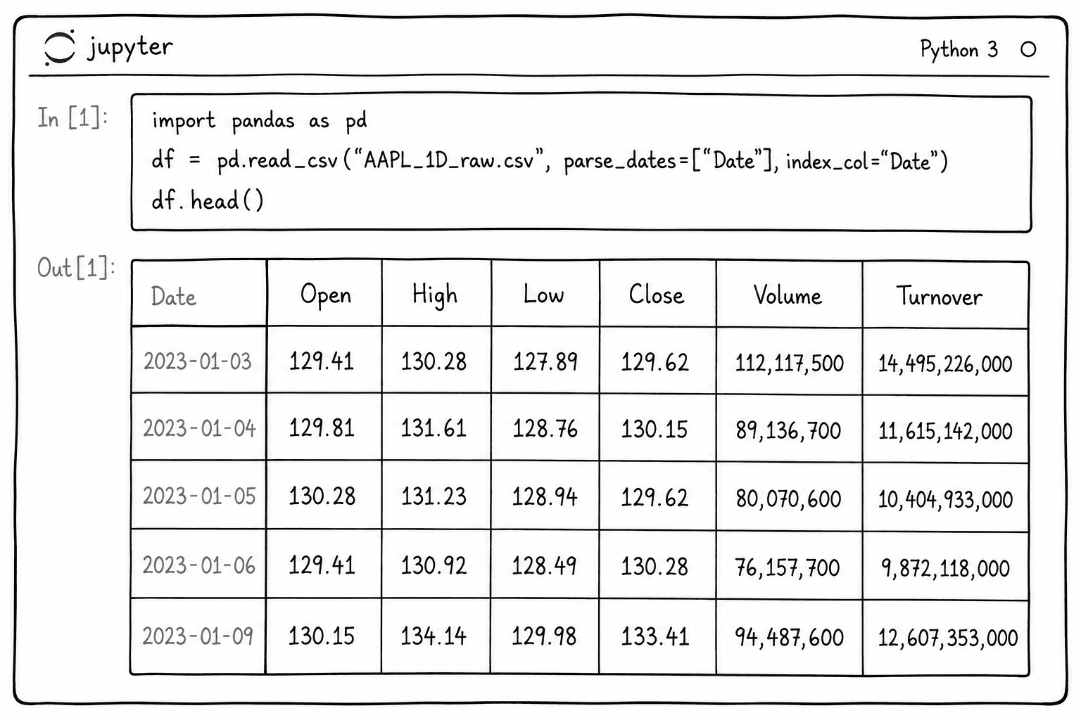
Starting small. The notebook first downloads price data for a few well-known tickers (AAPL, TSLA, GOOG) so you can see how the Norgate API works. It uses total-return-adjusted prices, which account for dividends and stock splits, and returns a clean pandas DataFrame with OHLCV columns.
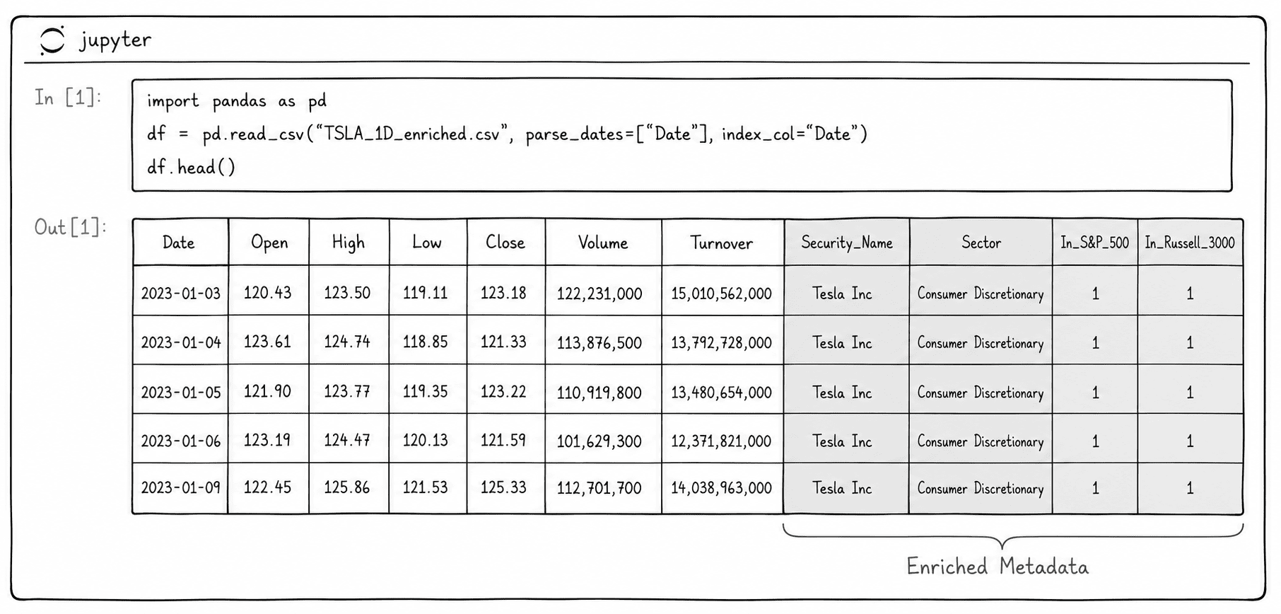
Enriching with metadata. Once you have the raw prices, the notebook adds three layers of information to each row:
Company name using Norgate’s security name lookup. Adds a
Security_Namecolumn (e.g., “Apple Inc”).GICS sector using the Global Industry Classification Standard. Adds a
Sectorcolumn (e.g., “Information Technology”).Index membership using Norgate’s index constituent time series. Adds
In_S&P_500andIn_Russell_3000columns as binary flags (1 = member on that date, 0 = not).
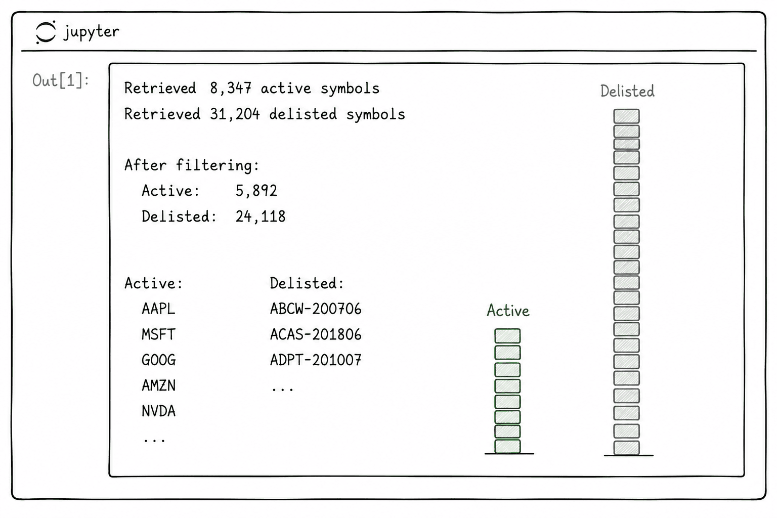
Scaling to the full market. The notebook then retrieves every symbol from both the US Equities and US Equities Delisted databases, filters to equities only (excluding ETFs, REITs, etc.), and runs the same enrichment pipeline across the entire universe.
Merge and export. Finally, active and delisted data are combined into a single DataFrame, sorted by date, and saved as a .parquet file.
What You Get
A single .parquet file containing every U.S. equity, active and delisted, with daily OHLCV prices, company names, GICS sectors, and point-in-time S&P 500 and Russell 3000 membership flags. Ready for backtesting.
Part 2: Point-in-Time Index Membership Tables
Why This Matters
Even with a survivorship-bias-free price database, there is another subtle bias that can distort your backtests: index membership bias.
If you want to backtest a strategy on “S&P 500 stocks,” which S&P 500 do you use? Today’s constituents? That is the wrong answer. The S&P 500 composition changes constantly. Companies are added when they grow large enough and removed when they shrink, get acquired, or go bankrupt. Using today’s list to represent the past means you are implicitly selecting stocks that performed well enough to remain in the index.
What you actually need is a point-in-time record: on January 15, 2018, which exact stocks were in the S&P 500? On March 3, 2020? The answer is different for every date.
What the Notebook Does
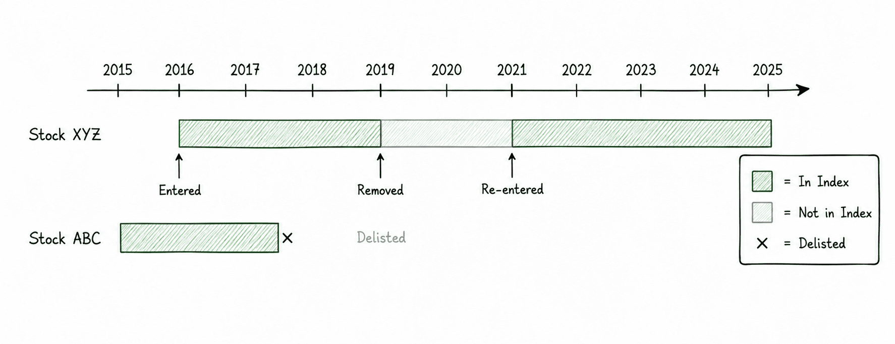
The core concept is membership spells: continuous periods during which a stock belongs to an index. A stock can have multiple spells if it was removed and later re-added.
Configuration. You define which indices to analyze (e.g., $NDX for Nasdaq 100, $SPX for S&P 500) and the date range. The notebook explains how to look up the correct Norgate symbol codes using their Data Viewer tool.
Symbol universe. The notebook pulls all active and delisted U.S. equity symbols, because restricting to currently active stocks would reintroduce survivorship bias.
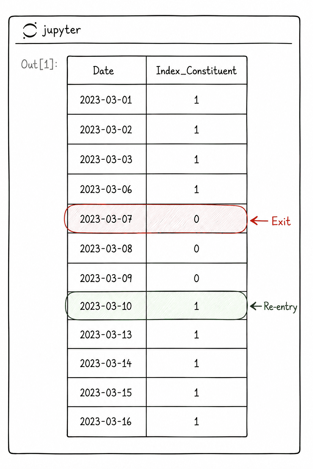
Spell detection. For each symbol and index pair, the notebook retrieves the daily index constituent time series from Norgate (a binary 1/0 signal indicating membership on each date) and scans it sequentially. When a stock enters the index, a new spell begins. When it leaves, the spell ends on the last day the stock was still a member.
A few design decisions worth noting:
Pre-existing members (stocks already in the index on the start date) get a blank entry date, since the algorithm cannot determine the original entry from within the window.
Exit date is the last day the stock was still in the index, not the first day it dropped out.
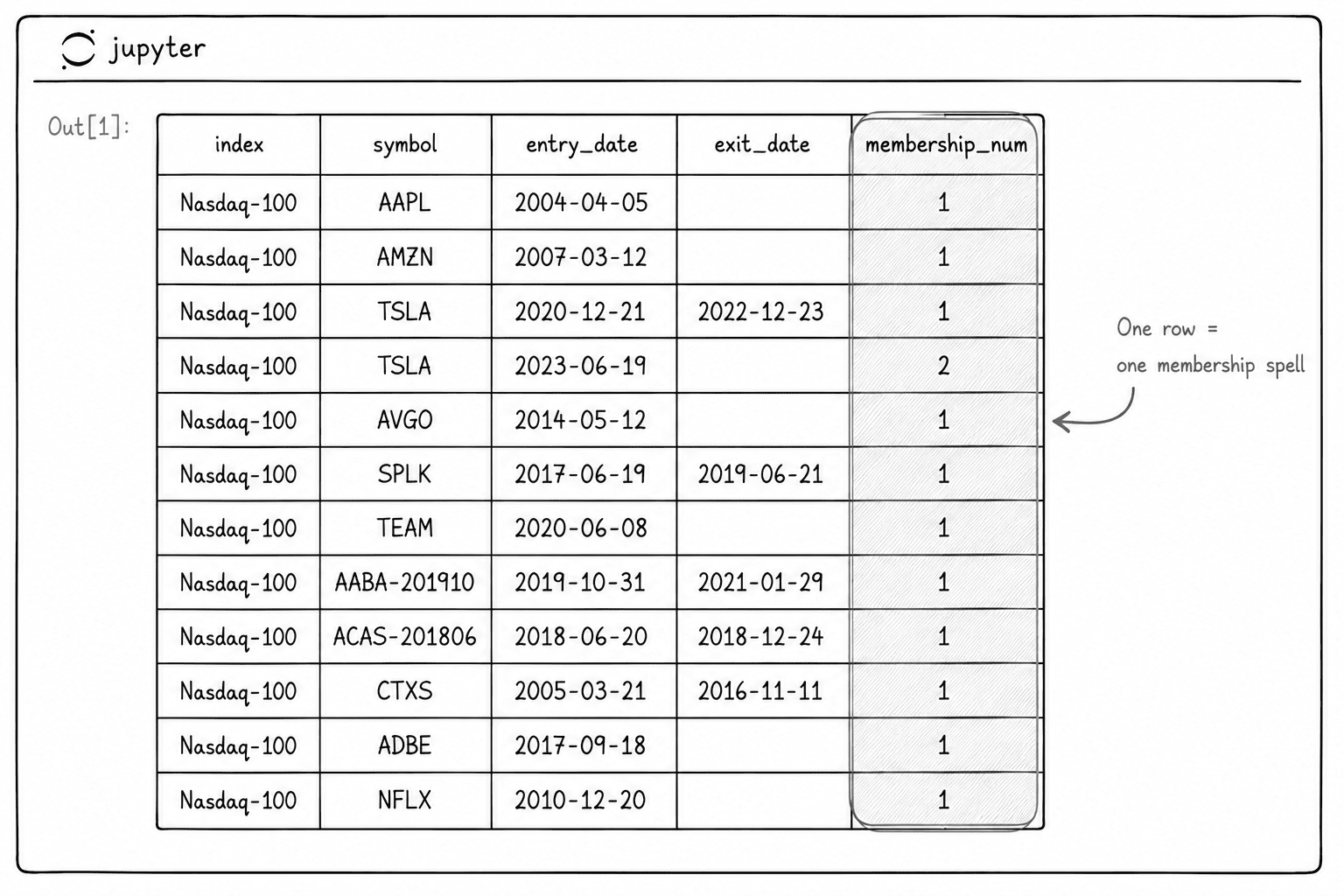
A membership counter tracks re-entries: a stock with membership number 2 entered the index, was removed, and entered again.
Full scan. The notebook runs this function across every symbol in the entire U.S. equity universe for each configured index. Scanning approximately 40,000 symbols per index takes about 4 to 5 minutes each. The results are combined into a single DataFrame and exported as CSV.
What You Get
A CSV file (e.g., ndx_spx_constituents_2015_2025.csv) containing one row per membership spell. Each row tells you exactly when a stock entered and exited a specific index. This file can be directly joined with your price data to filter your backtest to only the stocks that were actually in the index on each date.
Part 3: Complete Futures Database Pipeline
Why This Matters
Futures data is fundamentally different from equity data. You are not dealing with one continuous time series per instrument. You have dozens or hundreds of individual contracts per market, each with its own expiry date, and you need to stitch them together into continuous series while keeping track of which specific contract you are in at any given time.
Getting this wrong leads to phantom P&L from roll gaps, incorrect position sizing from using adjusted prices for dollar calculations, and missed roll signals from ignoring volume transitions between contracts.
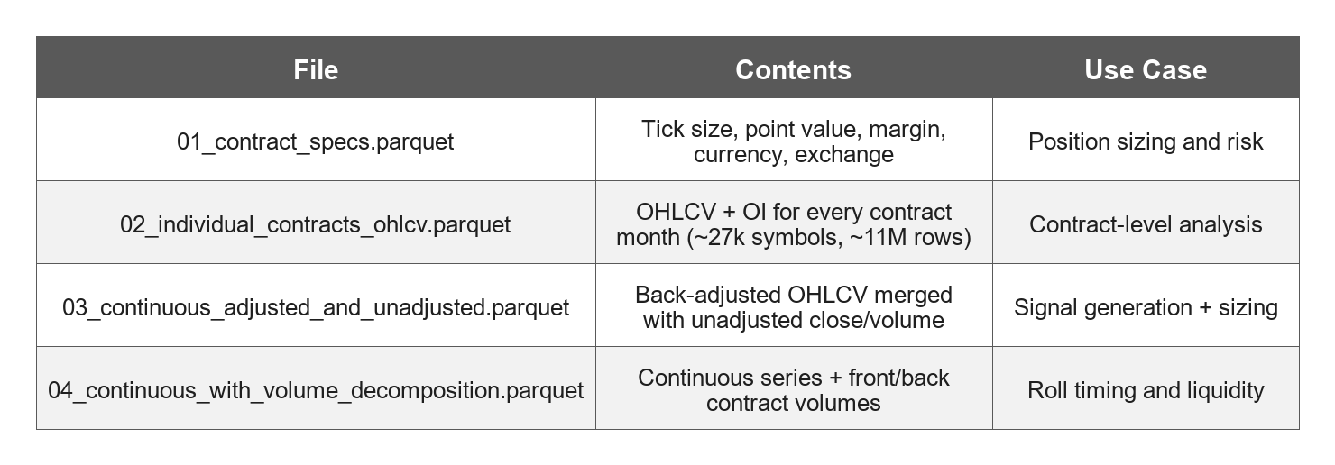
This workflow builds four Parquet files that cover the full spectrum: from raw contract metadata to a fully enriched continuous series with volume decomposition.
What the Notebook Does
The notebook produces four Parquet files, each building on the previous one.
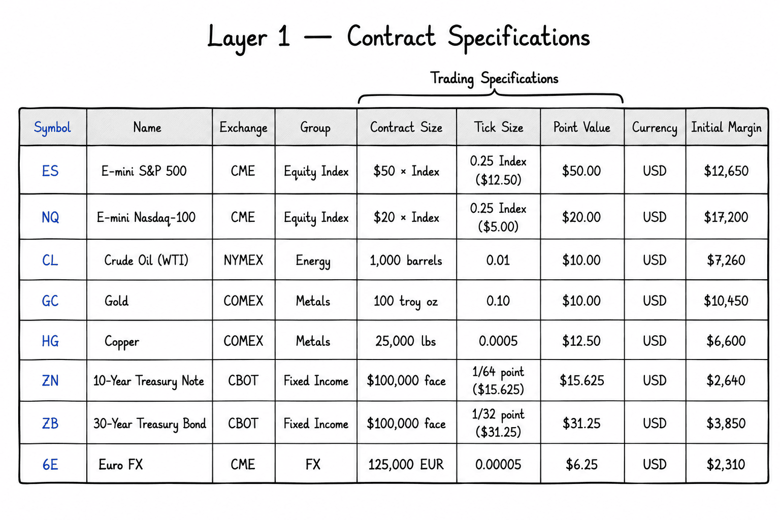
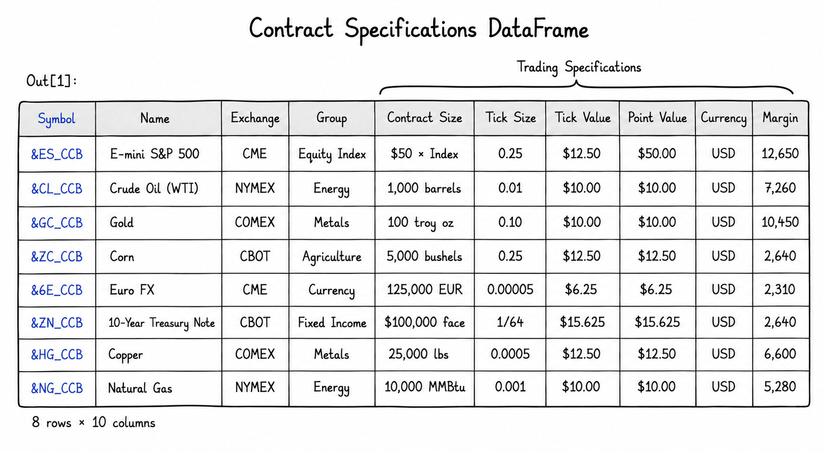
Layer 1: Contract Specifications. The pipeline starts by pulling metadata for every futures market: tick size, point value, margin requirements, currency, exchange, and classification group. This is the foundation for position sizing and risk calculations.
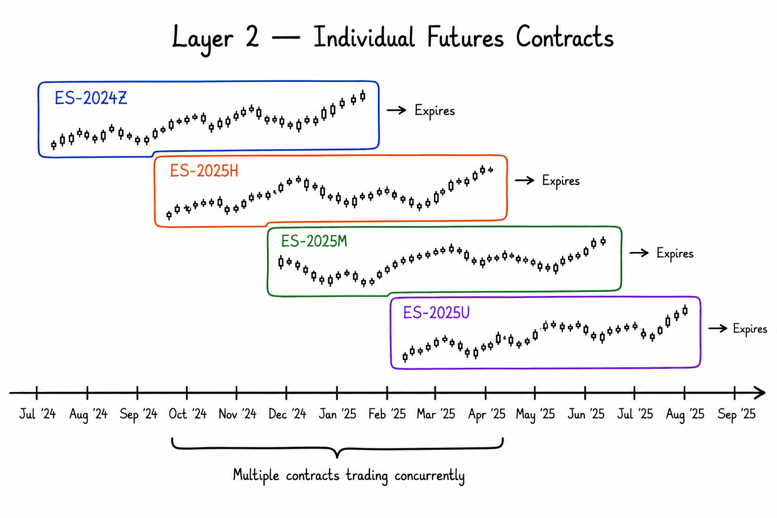
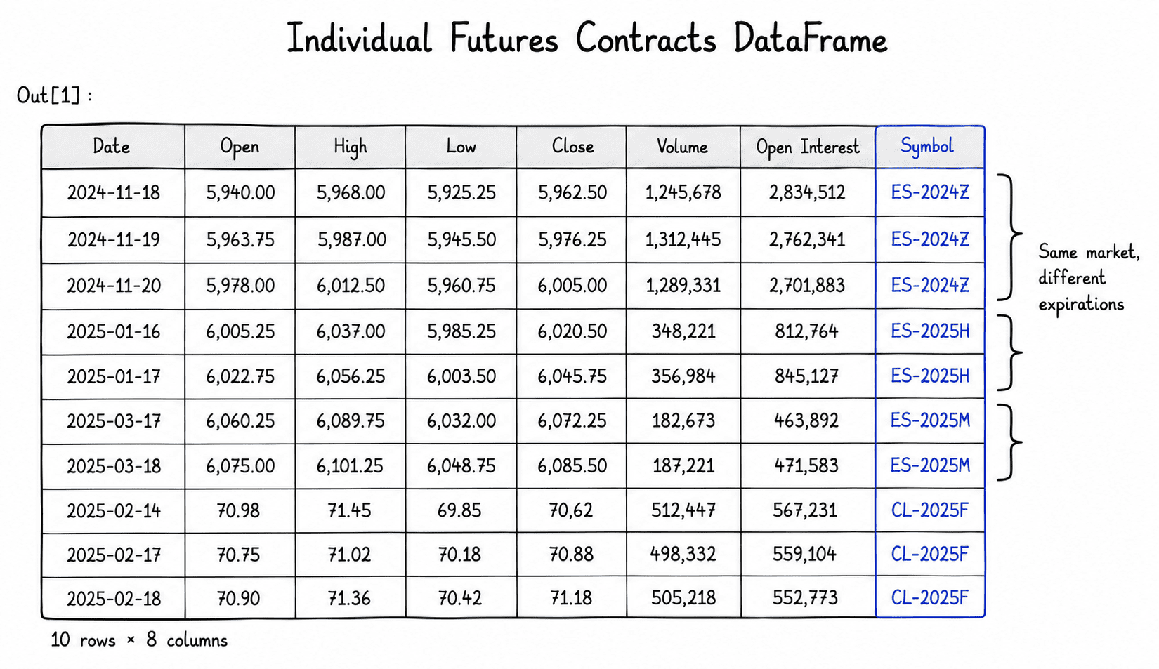
Layer 2: Individual Contracts. All individual futures contracts are then downloaded, including expired ones. Each contract is queried for its full OHLCV series with open interest. The download runs in parallel with 10 workers since there are roughly 27,000 individual contract symbols producing around 11 million rows.
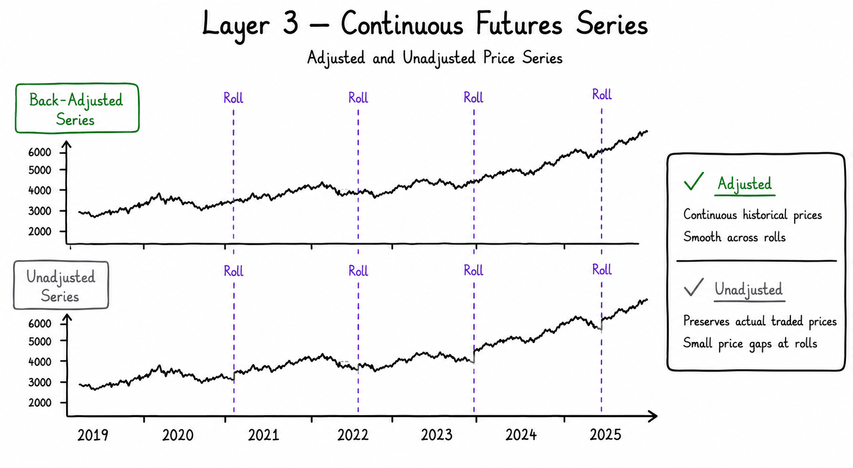
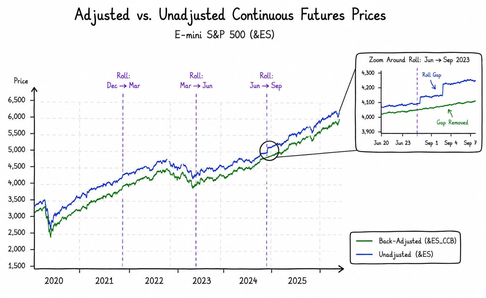
Layer 3: Continuous Adjusted and Unadjusted Series. This is where it gets subtle. Norgate provides two types of continuous symbols for each market:
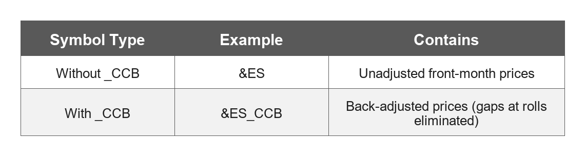
You need both. Adjusted prices for signal generation (no artificial jumps at roll dates) and unadjusted prices for position sizing (real dollar values). The notebook merges them into a single row so each date has both representations available.
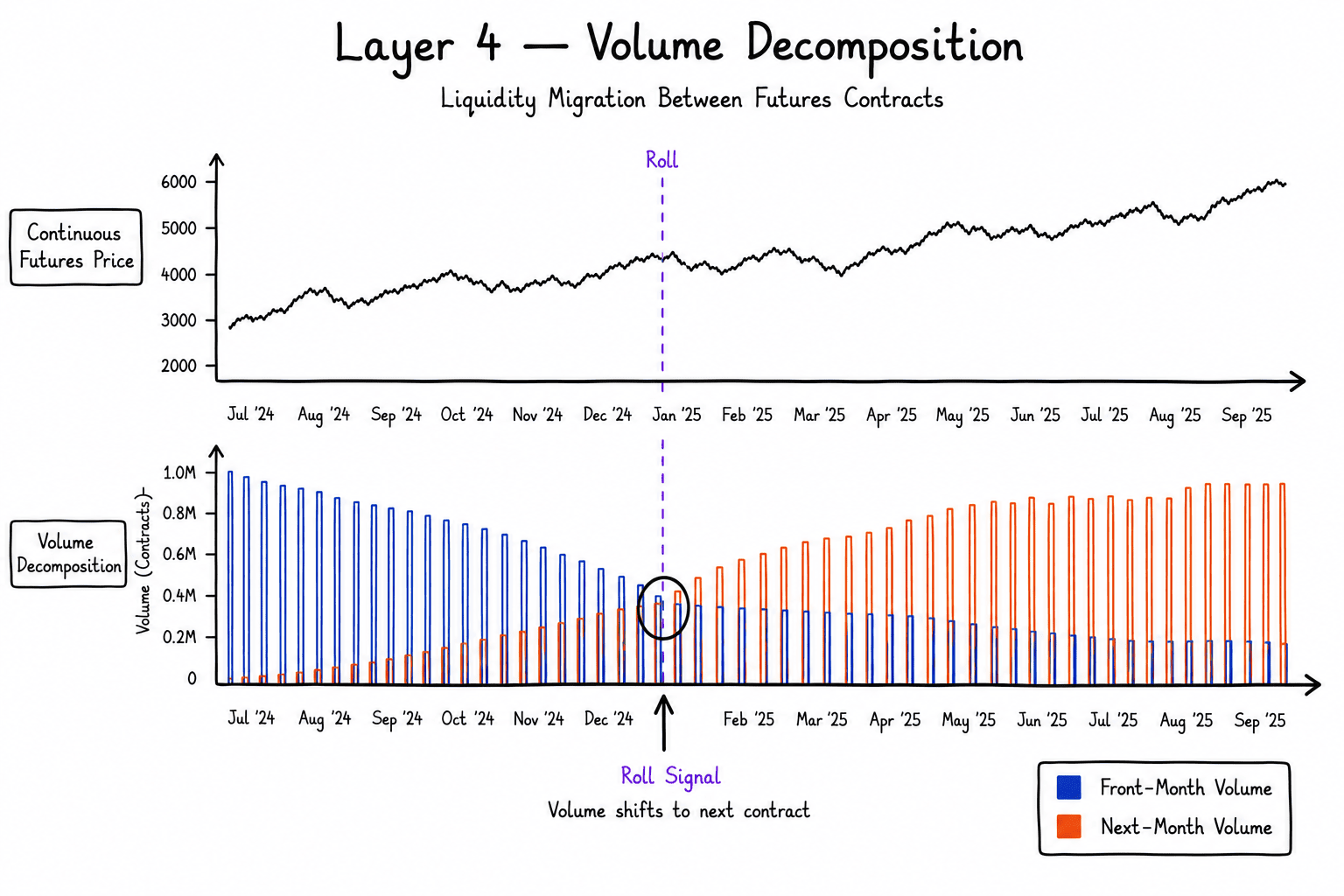
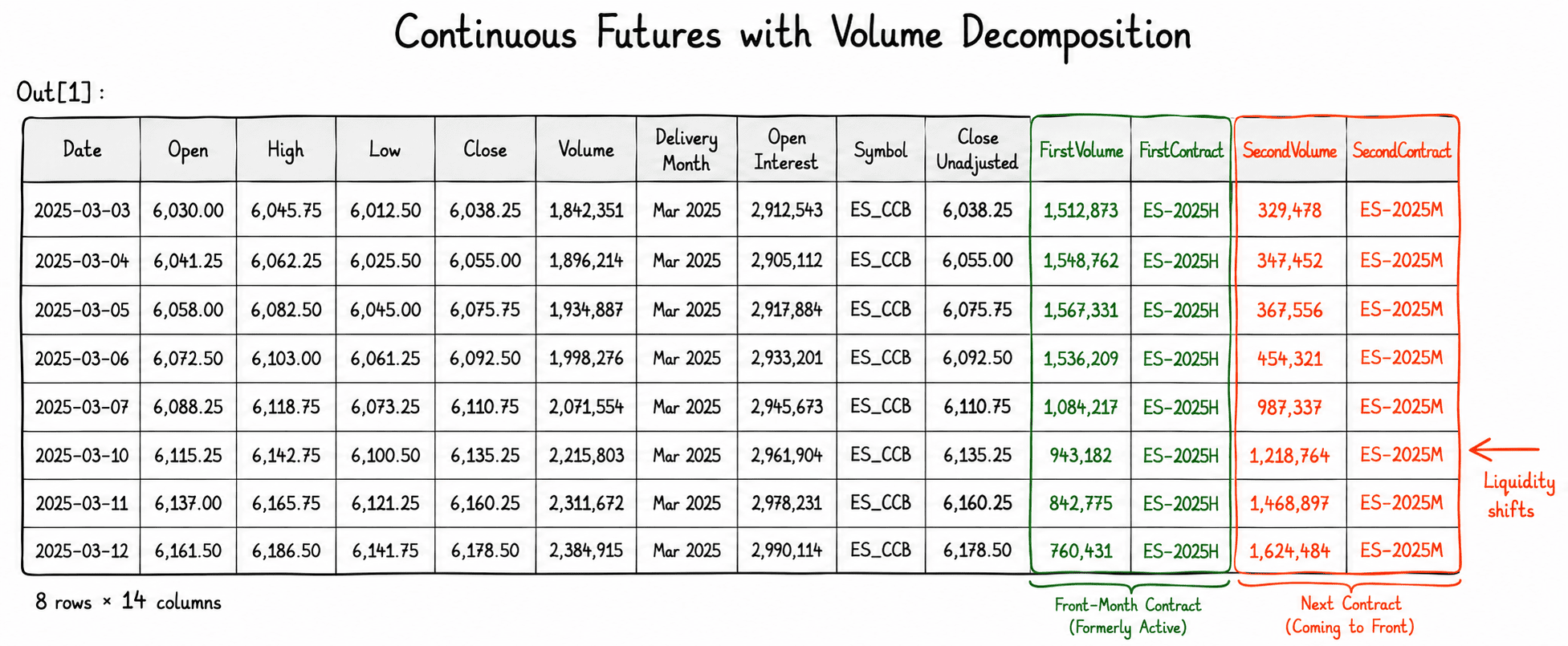
Layer 4: Volume Decomposition. The final layer enriches the continuous series with volume from the first-to-expire and second-to-expire contracts, which (as volume shifts from the front-month to the next contract) is critical for understanding proper roll dynamics.
The pipeline parses individual contract symbols (e.g., ES-2025M) to determine expiry dates, builds a sorted map of contracts per commodity, and then for each date finds the two nearest active contracts and records their volumes.
What You Get
Four Parquet files in the norgate_output/ directory:
Download and Run
All three workflows are provided as Jupyter notebooks alongside this article. Download them, adjust the configuration in the first cell (date range, indices, output paths), and run.
Each notebook includes its own setup instructions and prerequisites.
Conclusion
Data quality is not glamorous, but it determines whether your research conclusions are real or artifacts. Survivorship bias, index membership bias, and incorrect futures roll handling are three of the most common ways backtests can lie to you.
These three workflows address each of those problems directly. They produce clean, structured, Parquet-based datasets that you can plug into any backtesting framework or research pipeline.
Download the notebooks, run them, adapt them, and build on them.
Disclaimer
This publication is provided by Concretum Group for informational, educational, and research purposes only. It does not constitute investment, financial, legal, or tax advice, nor a recommendation to buy or sell any security, instrument, strategy, or investment product. All investments involve risk, including possible loss of principal. Past performance, backtested performance, and historical analysis are not reliable indicators of future results. Readers should conduct their own research and consult qualified professionals before making investment decisions.
Full disclaimer: https://concretumgroup.com/disclaimer/