

Automating a Volatility Strategy With Python and Interactive Brokers
From Research Paper to Live Execution

A few months ago, we published a research paper called The Volatility Edge: A Dual Approach For VIX ETNs Trading.

It won 5th place at the Quantpedia Awards 2026. The strategy compounds at 16.3% per year over a 17-year backtest, delivers a Sharpe ratio of 1, and keeps equity market correlation near 15%.
This article shows how to build an automated VIX volatility trading strategy using Python and Interactive Brokers. Based on our award-winning research, the strategy seeks to capture the volatility risk premium through systematic exposure to VIX-linked ETNs.
The paper is public. The strategy rules are fully transparent. And we built a Python notebook that automates the entire thing through Interactive Brokers.
This article is about the process of turning a research idea into a working automated trading system. We walk through the theory behind the strategy, the signal logic, the position sizing, and the code that connects it all to a live broker API.
This is meant as an educational exercise, not a production-ready system. The notebook is a starting point. We strongly encourage anyone interested to run their own tests, validate the signals on out-of-sample data, and stress-test the execution logic before deploying any real capital. The goal here is to show what the workflow looks like, not to hand you a finished product.
Let’s start with the theory.
Why Volatility Is Tradable
Most investors bet on direction. They buy stocks hoping prices go up, or they short hoping prices go down. Volatility traders don’t care about direction. They bet on how much prices will move, regardless of which way.
In practice, this means buying volatility when it’s cheap (usually when the crowd is calm) or selling volatility when participants are willing to overpay for it (usually when fear dominates and everyone wants portfolio insurance).
The key insight is simple: implied volatility, what the options market thinks will happen, almost always overestimates what actually happens. The VIX Index, which represents the market’s 30-day volatility forecast for the S&P 500, has overestimated realized volatility roughly 80% of the time over the past two decades.
That gap between what the market expects and what actually unfolds is called the Volatility Risk Premium (VRP).
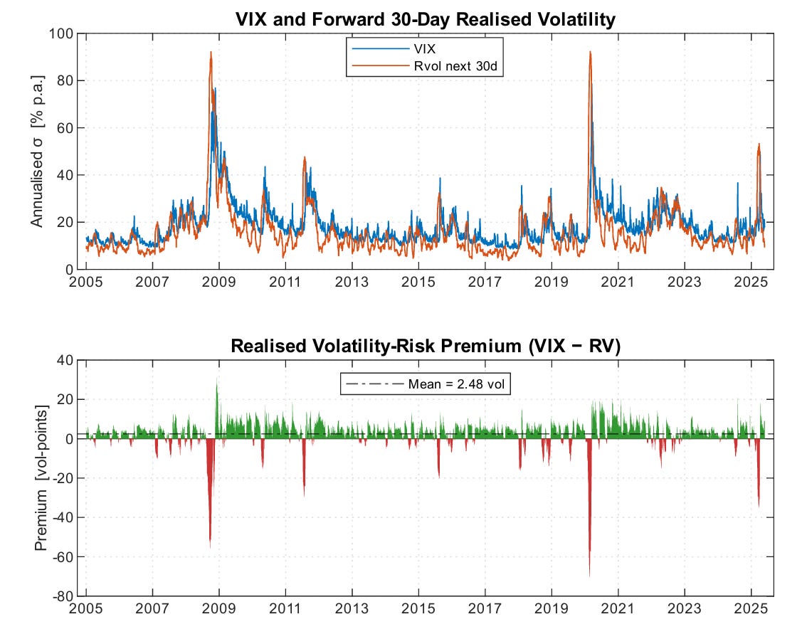
Why does this premium exist? Because volatility tends to spike when equities fall. Portfolio managers buy protection through options and variance swaps, and the pool of risk-averse buyers persistently exceeds the pool of sellers willing to warehouse that risk. In equilibrium, sellers demand a premium. That premium is what we’re trying to capture.
From Variance Swaps to VIX ETNs
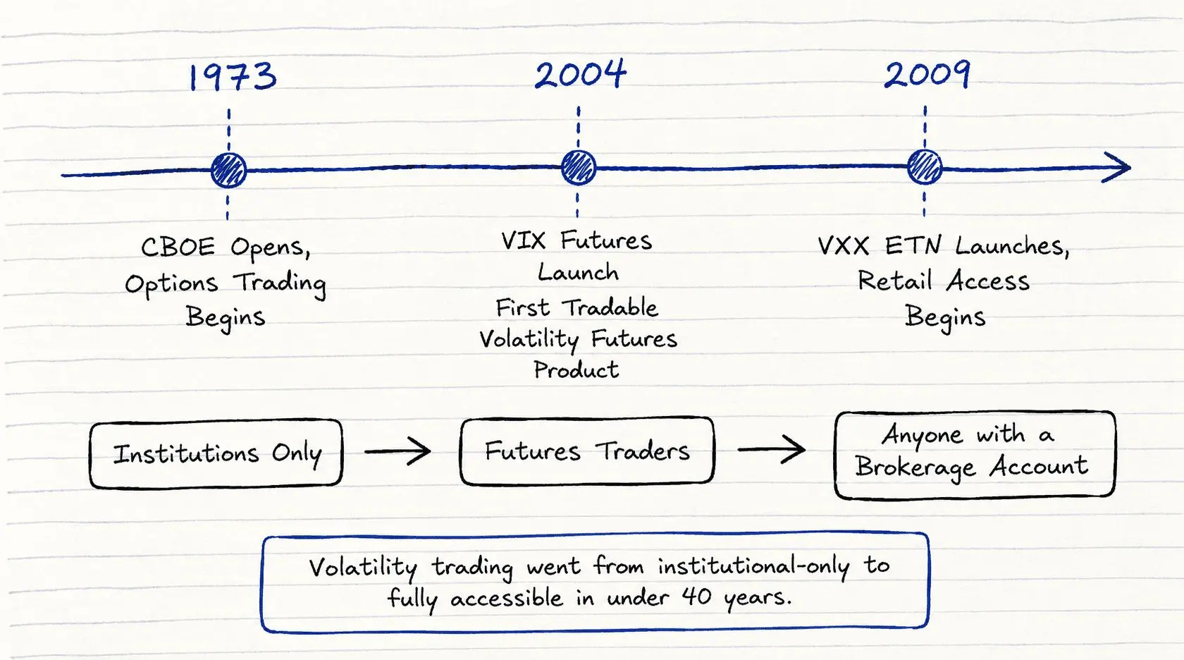
For decades, the only way to trade volatility directly was through variance swaps. These are OTC contracts between institutions, requiring ISDA agreements, large notionals, and counterparty infrastructure. Not exactly accessible to individual investors.
That changed in March 2004, when VIX futures launched on the Cboe Futures Exchange. And it changed again in January 2009, when Barclays launched VXX, the first exchange-traded note linked to VIX futures.
Suddenly, anyone with a brokerage account could trade volatility.
VXX tracks a rolling position in the two nearest-month VIX futures contracts, maintaining an average maturity of about 30 days. Think of it as a daily rolling bet on short-term VIX futures.
Today, several VIX-linked products exist:
VXX / VIXY: Long volatility (1x exposure to 30-day VIX futures)
SVXY: Short volatility (-0.5x inverse exposure)
UVXY / UVIX: Leveraged long volatility (1.5x or 2x)
SVIX: Short volatility (-1x inverse exposure)
The strategy in the paper uses SVXY to go short volatility and VXX to go long volatility. That’s it. Two instruments, one brokerage account.
The Dual Signal
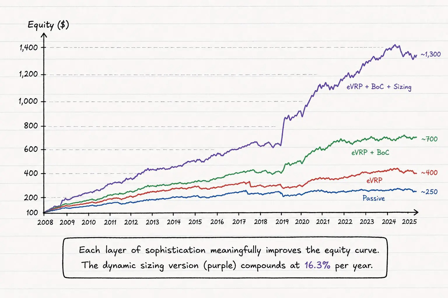
The paper builds up to the final strategy through four progressive versions. Each one adds a layer of sophistication. We’ll skip straight to the logic that matters: the two signals that drive the final strategy.
Signal 1: Expected Volatility Risk Premium (eVRP)
This answers a simple question: is implied volatility currently higher or lower than what we expect realized volatility to be?
To estimate future realized volatility, we compute the standard deviation of the last 10 daily SPY returns and annualize it:
eRV30 = std(last 10 daily returns) * sqrt(252) * 100Then we compare it to the VIX:
eVRP = VIX - eRV30If eVRP is positive, the market is pricing in more volatility than recent history suggests. The premium looks attractive. If eVRP is negative or zero, the market might be underpricing risk, and shorting volatility becomes dangerous.
Signal 2: VIX Term Structure (Backwardation or Contango)
This answers a different question: what does the shape of the VIX curve tell us about market stress?
We compare the VIX (30-day implied volatility) to VIX3M (90-day implied volatility):
VIX < VIX3M (Contango): The market expects calmer conditions in the near term. This is the normal state. Uncertainty naturally increases with time horizon.
VIX > VIX3M (Backwardation): The market expects more volatility in the near term than in the medium term. This signals stress.
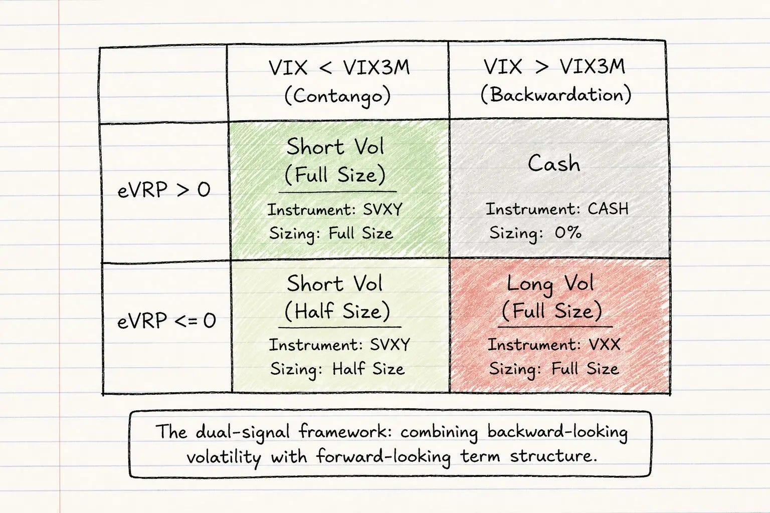
Combining these two signals gives us four regimes:
1. eVRP > 0 and VIX < VIX3M: Best case. The premium is attractive and the term structure is normal. Go short volatility at full size.
2. eVRP <= 0 and VIX < VIX3M: The premium has compressed, but the term structure is still calm. Stay short volatility, but at half size.
3. eVRP <= 0 and VIX > VIX3M: Both signals are negative. The expected premium is gone and the term structure is inverted. Flip to long volatility.
4. eVRP > 0 and VIX > VIX3M: Mixed signal. The premium looks attractive but the term structure says stress. Stay in cash.
Dynamic Sizing
Here’s where the strategy gets clever.
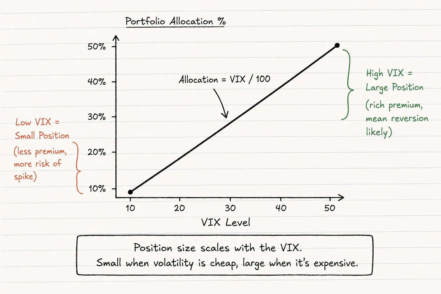
A static allocation to short volatility is dangerous because the risk of shorting volatility is not constant. When the VIX is at 12, even a modest shock can cause it to double. You collect small premiums while sitting in front of a steamroller. When the VIX is at 35, the odds of it doubling again are much lower, and the premium you’re getting paid is much richer.
The paper uses a dead-simple sizing rule: your allocation equals the VIX level divided by 100.
VIX at 15? Allocate 15% of your portfolio.
VIX at 30? Allocate 30%.
VIX at 50? Allocate 50%.
This naturally reduces exposure during fragile low-VIX environments and increases it when volatility is elevated and the expected payoff is higher.
The full strategy rules are:
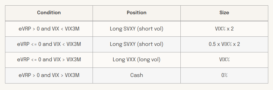
The “x 2” on SVXY is because SVXY only provides -0.5x exposure. To get the equivalent of a -1x short, you need twice the dollar amount.
The portfolio is rebalanced only when the current allocation drifts more than 2% from the target. This avoids unnecessary trading and keeps transaction costs low.
The Results
Over the January 2008 to May 2025 backtest period, after 5 basis points of transaction costs per trade:
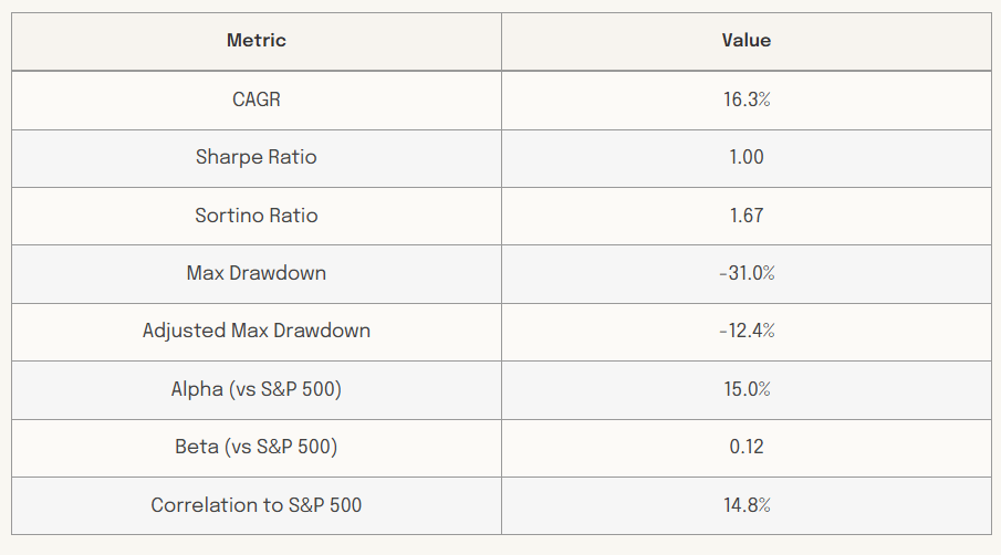
The strategy was short volatility on 90% of days, in cash for 6%, and long volatility for 4%.
What makes these numbers interesting is the combination: high absolute returns, near-zero correlation to equities, and a Sharpe of 1. Blending even a 10-20% allocation of this strategy into a passive SPY portfolio boosts the combined Sharpe ratio by roughly 20%.
Automating It
The strategy runs once per day, near the close.
The execution method is a Market-on-Close (MOC) order. A MOC order is submitted before the exchange cutoff (typically 3:50 PM ET on the NYSE) and gets executed at the official closing auction price. You don’t control the exact price, but you get the close, which is the most liquid print of the day. This is what institutional rebalancing flows use, and it’s the execution method assumed in the paper’s backtest.
Because MOC orders must be submitted before 3:50 PM, we need the signal ready before that deadline. The system computes signals at 3:45 PM ET. More precisely, it uses the closing price of the 1-minute bar that starts at 3:44 PM, which represents the market state at 3:45. This gives enough time to fetch data, compute the signal, and submit the MOC order before the cutoff, with a few minutes of buffer.
So the daily workflow is: at 3:45 PM ET, grab three numbers (VIX, VIX3M, and the 10-day realized volatility of SPY), compute the signal, determine the position size, and submit a MOC order. That’s it.
The full automation pipeline has four steps.
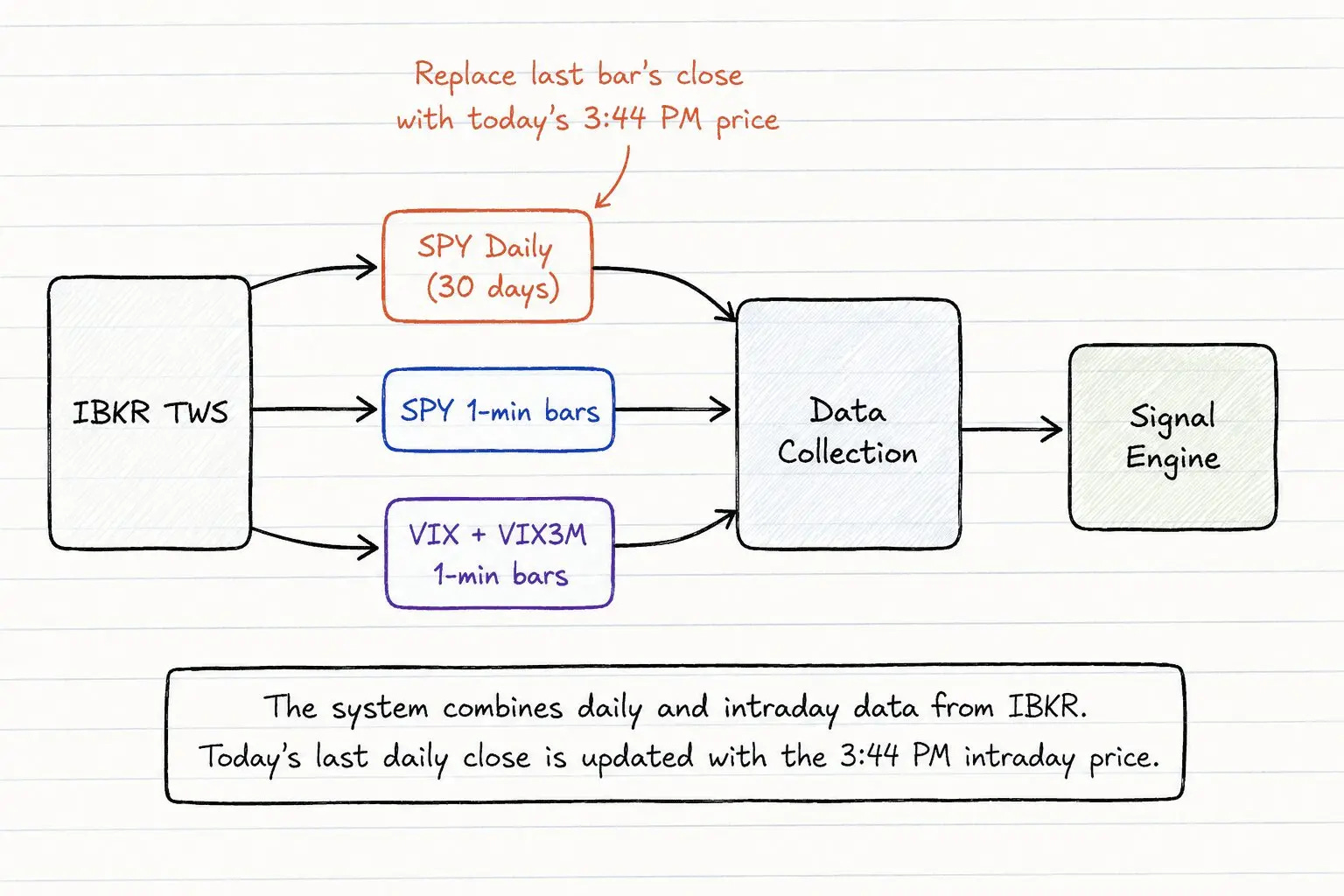
Step 1: Connect and Fetch Data
The system connects to IBKR’s Trader Workstation via the ib_async Python library. It pulls 30 days of daily SPY closes and one day of minute-level data for SPY, VIX, and VIX3M.
The last daily SPY close gets replaced with the 3:44 PM intraday price, so the realized volatility estimate includes today’s move up to the signal time.
Step 2: Compute the Signal
Using the data from Step 1:
Compute the 10-day standard deviation of SPY returns, annualize it
Subtract it from the current VIX to get eVRP
Compare VIX to VIX3M to determine contango or backwardation
Map the two signals to one of the four regimes
Step 3: Size and Place Orders
Once the signal is determined:
Compute the target allocation using VIX / 100
Convert that to a dollar amount based on account equity
Divide by the current price of SVXY or VXX to get share count
Compare the target weight against the current weight
If the difference exceeds the 2% rebalancing threshold, submit a MOC order
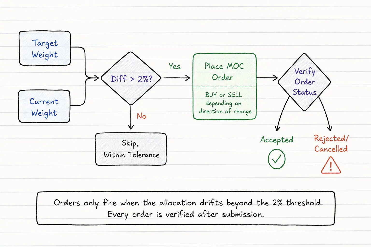
Step 4: Log and Disconnect
Every execution is logged to a CSV file with the full state: prices, signals, weights, target positions, orders placed, and timestamps. The system then disconnects from IBKR.
The Code
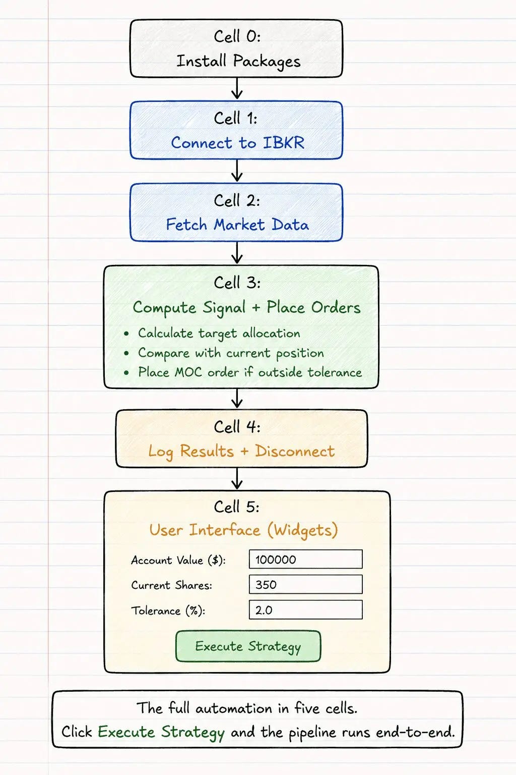
The full implementation is a Jupyter notebook with five cells. Here’s the structure:
Cell 0: Install packages. ib_async, pandas, numpy, pytz, ipywidgets.
Cell 1: Setup. Connects to IBKR, qualifies the five contracts (SPY, VIX, VIX3M, VXX, SVXY).
Cell 2: Data collection. Waits until the signal time, fetches daily and intraday data, extracts the 3:44 PM prices.
Cell 3: Signal and execution. Computes eVRP, checks term structure, determines sizing, fetches live prices for VXX/SVXY, calculates target shares, compares against current holdings, places MOC orders if the rebalancing threshold is breached, and verifies order acceptance.
Cell 4: Logging. Writes every field to a CSV and disconnects.
Cell 5: User interface. A widget-based form where you enter your account value, current positions, market close time, and rebalancing threshold. One click runs the entire pipeline.
The notebook is publicly available. You can find it in the Google Colab link referenced in the paper.
Running It in Practice
A few things to keep in mind before you run this live.
Use paper trading first. Connect to IBKR’s paper trading account (port 7497) and run the strategy for a few weeks. Watch the signals, verify the orders, check the CSV log. Make sure the numbers make sense before you risk real capital.
Update your positions precisely. The current version takes your VXX and SVXY share counts as manual input. If you enter the wrong numbers, the orders will be wrong. Double-check before every execution.
Respect the MOC deadline. Market-on-Close orders must be submitted before 3:50 PM ET on the NYSE. The strategy computes signals at 3:44 PM and submits immediately after. That gives you a comfortable window, but don’t add unnecessary delays.
Watch for early-close days. A handful of trading sessions each year close at 1:00 PM ET instead of 4:00 PM. The notebook lets you adjust the market close time via a dropdown. On those days, select the 13:00 option so the signal time shifts to 12:44 PM and the MOC order goes out before the early cutoff.
This is not a set-and-forget system. The strategy is systematic, but the execution environment needs supervision. Connections drop, data goes stale, orders get rejected. If you want to learn more about what can go wrong, we wrote a separate article on Building Reliable Algo Trading Systems.

Conclusion
Volatility trading used to be the exclusive domain of institutional hedge funds with OTC infrastructure, ISDA agreements, and dedicated quant teams. That’s no longer the case.
With a standard brokerage account, two ETNs, and a few lines of Python, individual investors can now access the same volatility risk premium that institutions have harvested for decades. The strategy presented here is deliberately simple: two signals, dynamic sizing, and one daily trade. No options expertise required. No leverage. No complex hedging.
The full research paper is available publicly. The code is open source.
But simplicity does not mean safety. Volatility itself is volatile. Position sizing matters. Risk management matters. And the operational details of running live automated systems matter just as much as the strategy logic.
Use the paper as a starting point. Study the signals. Run the notebook on paper trading. Understand what you’re doing before you deploy capital. And if you need help building a more robust production setup around it, reach out.
If you found this article useful, feel free to leave a comment and reach out via direct message or email at info@concretumgroup.com for any questions.

Disclaimer
This publication is provided by Concretum Group for informational, educational, and research purposes only. It does not constitute investment, financial, legal, or tax advice, nor a recommendation to buy or sell any security, instrument, strategy, or investment product. All investments involve risk, including possible loss of principal. Past performance, backtested performance, and historical analysis are not reliable indicators of future results. Readers should conduct their own research and consult qualified professionals before making investment decisions.
Full disclaimer: https://concretumgroup.com/disclaimer/